iNat Isn't Slowing Down in Arizona

The iNaturalist website collects species observations from people all over the world.  It started in 2008 and grew slowly at first and then entered a period of rapid growth in 2017.  As a consequence, the number of species recorded on the website is constantly increasing, passing 300,000 in 2020.  The website is currently adding more than 50 million observations a year. This raises an interesting biodiversity question: how long can the number of species keep increasing?  Another way of stating the question: how many species are there?

Biodiversity scientists use species accumulation curves to estimate the total number of species in a given area.  As they investigate a new study site, they record new species and the date/time the species was observed.  For most sites, the number of new species increases rapidly as scientists describe common species; the number of new species slows as scientists search for more and more rare species.  Graphing the number of species over time should reveal a logarithmic curve.  Based on the equation for that curve, scientists can estimate the asymptote - the number of species the curve will eventually reach given enough time.  This allows scientists to estimate the total number even if they don't finish counting all of the species.

This slowing down does seem to be happening for total species count on iNat.  For example, the 2024 Year in Review showed 50 million observations over the year, and about 1,000 new species (not previously observed and posted to iNat) per month.  

From iNat 2024 Year in Review

In contrast, back in May 2019 more than 6,000 new species were added.  It appears that 2019-2020 was the peak for adding new species, and even as more new users have joined iNat, fewer and fewer new species are being observed.  

These charts show running totals, with new additions colored, so that the logarithmic curve is more visible in Newly Added Species:

From 2024 Year in Review

There were fewer observations and many fewer users in 2019-2020, than now, but the rate of newly added species was much greater.  This appears to indicate that it is getting harder and harder to find new species to add to iNat.  Observable species on iNat are those that can be distinguished with photographic evidence, usually limited to smartphone cameras.  So this estimate does not include microbial life, and probably excludes most microscopic life.  

Its possible that unobserved species are mostly in the middle of remote wilderness areas and that is why fewer and fewer are being observed.  But many of the new species are from the US and Europe - there's still lots to explore!

For example, in Arizona the species accumulation curve is still effectively linear, with about 700 new species each year.  No signs of slowing down here!

The same is true of smaller areas within AZ, for example the Prescott National Forest averages 186 new species observed each year.  

I considered whether the new species could be due to rare birds and insects showing up for the first time.  I also analyzed new plant taxa on Coconino National Forest.  Plants are well-studied and the forest has been extensively surveyed, so it seems unlikely that new species would be discovered yearly.  But, according to the iNat data, not only are new species being continuously discovered, there is no detectable slow down in the rate of discovery!

I'm not sure what conclusions to draw from this analysis.  The standard conclusion would be that we haven't sampled enough species yet to begin to see the rate of new species discoveries slowing down.  This implies that the total number of species is quite a bit greater than the number that have been recorded so far on iNat.  

Another interpretation could be that the actual number of species isn't constant.  In other words, there could be new plants showing up each year on the Coconino.  This could be due to new invasive species, shifting distributions of native species.  It could also be impacted by taxonomist naming conventions; the number of species in even well-explored areas could increase as botanists work to name and describe the huge floristic diversity of the world.

There is still a lot of biodiversity to explore, even in our backyards!

Acid-Base Balance: Foods and Supplements

I previously wrote about the role lactic acid can play in disease.  This raised the question of whether foods and supplements can buffer metabolic acidity.  If so, which foods or supplements are most beneficial?  Does pH correlate to the effect on the acid-base balance of the body?

This is important because:

• Chronic acid load can deplete alkalinizing minerals, leading to e.g. calcium bone loss.
• Long Covid may be caused by metabolic acidosis: https://researchaidnetworks.org/hypothesis-summary/

After researching this, I concluded that a food's pH does not directly correlate with its impact on overall acid base balance.  Potential Renal Acid Load (PRAL) is determined by mineral and protein composition, not its inherent acidity.  

For example:

• Lemons taste acidic due to citric acid, but have a negative PRAL (alkaline-forming) because they're rich in potassium and other compounds that generate bicarbonate when metabolized
• Animal proteins may not taste acidic but have a high positive PRAL (acid-forming) due to sulfur-containing amino acids that get metabolized to sulfuric acid.

The key biochemical factors that determine a food's PRAL include:

1. Protein content (especially sulfur amino acids) - metabolized to produce acids
2. Mineral content: 
1. Potassium, calcium, magnesium - metabolized to produce bicarbonate (alkaline)
2. Phosphorus, chloride - contribute to acid load
3. Organic acid content - intermediates in the citric acid cycle (Krebs cycle), their oxidation generates bicarbonate. Each molecule of malate or citrate metabolized can generate multiple bicarbonate molecules.

Details

The pH of urine is influenced by the body's metabolic acid load and the kidney's ability to regulate hydrogen ion (H⁺) excretion.  The kidneys play a crucial role in maintaining acid-base balance by adjusting the amount of hydrogen ions eliminated or retained.  When the body experiences a metabolic acid load, the kidneys respond by increasing H⁺ excretion. This lowers urine pH, reflecting the increased acid load on the body.  However, positive cations can also stimulate renal acid-base regulation, leading to increased hydrogen ion excretion (and bicarbonate (HCO₃⁻) regeneration).  This results in a decrease in urine pH, even as the body experiences a reduced metabolic acid load.

Cations can also activate enzymes that convert metabolic acids to bicarbonate.  The more positively charged the cation, the more efficiently it can displace hydrogen ions.

Organic acid conjugation to cations enhances alkalinization.  For example, citrate enters the citric acid cycle directly and generates multiple bicarbonate (HCO₃⁻) upon oxidation.

Table of Common Supplements and Food Additives; their pH and effect on acid-base balance.  

This data shows how solution pH and PRAL effects don't always correlate. For example, while KCl has a neutral pH in solution, it has a slightly negative PRAL due to the potassium content. However, extreme pH (either acid or base) can correlate with PRAL effect.

Categories of Supplements

1. Neutral pH, Alkalizing Effect: 
1. Potassium citrate
2. Calcium lactate
3. Potassium gluconate
4. These demonstrate the pH vs. physiological effect paradox
2. Mineral-Organic Complexes: 
1. Magnesium citrate and malate show slightly acidic pH but strong alkalizing effects
2. Zinc citrate has less alkalizing effect despite similar pH
3. Simple Salts: 
1. KCl shows neutral pH with mild alkalizing effect
2. NaCl shows neutral pH and neutral physiological effect
4. Strong Acids/Bases: 
1. HCl, KOH, NaOH show correlation between pH and physiological effect
2. These are exceptions to the general trend of pH not predicting physiological impact

Alkalinizing Potential Ranking

The formula for PRAL (mEq/100g) is: PRAL = 0.49 × protein (g) + 0.037 × phosphorus (mg) - 0.021 × potassium (mg) - 0.026 × magnesium (mg) - 0.013 × calcium (mg).  

Negative PRAL indicates an alkalizing effect on the body.

Example:  mice

Mice diets were compared using Dietary Cation Anion Balance (DCAB), a similar metric to PRAL.  DCAB is calculated by adding the weighted amount of acidifying anions and alkalizing cations in the diet. 

It has been shown in many species that the dietary cation anion balance (DCAB) influences acid base homeostasis and urine pH.  With the DCAB, the resulting urinary pH can be predicted with species-specific equations. 

DCAB [mmol/kg DM] = 49.9 · Ca + 82.3 · Mg + 43.5 · Na + 25.6 · K − 59.0 · P − 62.4 · S − 28.2 · Cl; mineral content in g/kg DM.  (Negative DCAB indicates an acidifying effect on the body.)

The paper found that a negative DCAB results in metabolic acidosis, and "Fed long-term, this can contribute to the reduction of bone mineral density due to a PTH-mediated increase in renal calcium excretion. Metabolic acidosis also induces renal phosphorus excretion, resulting in hypophosphatemia."

Citation: https://www.mdpi.com/2076-2615/11/3/702 

Böswald, L.F.; Matzek, D.; Kienzle, E.; Popper, B. Influence of Strain and Diet on Urinary pH in Laboratory Mice. Animals 2021, 11, 702. https://doi.org/10.3390/ani11030702

Example:  human athletes

Alkaline water has demonstrated its effectiveness as an alkalizing agent in the treatment of metabolic acidosis in both animal and human research. Past studies have shown that daily intake of 2.5–4 L of alkaline water for 3~6 weeks has significant impacts on anaerobic performance and acid–base balance in athletes.  This study showed that alkaline water co-ingested with glutamine led to decreased stress markers in athletes.  Masterjohn hypothesizes that glutamine is converted to glutamate to buffer lactic acid in muscles, and that decreasing PRAL contributes to more available glutamine for other metabolic functions..  

Citation: https://www.mdpi.com/2072-6643/16/3/454

Lu, T.-L.; He, C.-S.; Suzuki, K.; Lu, C.-C.; Wang, C.-Y.; Fang, S.-H. Concurrent Ingestion of Alkaline Water and L-Glutamine Enhanced Salivary α-Amylase Activity and Testosterone Concentration in Boxing Athletes. Nutrients 2024, 16, 454. https://doi.org/10.3390/nu16030454

Thanks to Claude Sonnet for back-and-forth conversation, and for creating the table and figure above.  

More Forest Thinning Science

1. You need Water for Ecohydrology

I previously wrote about the effects of thinning Southwestern ponderosa pine forests on forest hydrology.  AE Brown et al (Journal of Hydrology, 2005) summarized the last 50 years of hydrology research around the world on exactly this question.  Their conclusion was that yes, thinning increases water availability by decreasing evapotranspiration (ET).  However, at drier sites there is less of a difference.

In the figure above, the difference between the grass and forest curves represents the change in mean annual water yield for 100% conversion of one vegetation type to the other.  Partial conversion (i.e. thinning) was shown to have a proportional partial response.  The lack of difference between grass and forest in drier climates (below 500mm or 20 inches precipitation/year) indicates that most ET is actually just evaporation in these areas.  Therefore, because transpiration does not play a large role, reducing transpiration via thinning would not be expected to generate a large increase in water availability.

2. Don't Miss the Forest for the Trees

This classic forestry study found that thinning ponderosa forests increased growth of the remaining trees, but decreased total wood production.  In other words, the increase in vigor didn't compensate for the decrease in trees.  This even includes the decrease in disease (bark beetles) in thinned forests. So the question becomes, do you want a healthier forest or more wood?  

Data is from the The Level-of-Growing-Stock (LOGS) study on thinning ponderosa pine forests in the US West: A long-term collaborative experiment in density management.  A 2020 follow up provides a summary review of this study that started in 1962.  The The AZ portion of the study was conducted at Fort Valley experimental Forest just north of Flagstaff.   PDF with much more info is available from https://www.fs.usda.gov/rm/pubs/rmrs_p055.pdf.

Nutritional Yeast contains variable amounts of B vitamins

Nutritional yeast is tasty and nutritious!  How nutritious is it?  Well, that depends on whether it is fortified or not, and how much information you find on the nutrition label.  

After looking at the labels of about a dozen brands, I found that nutritional yeast is consistently a good source of B2, B3, and B5, and with fortification is a great source of all major B vitamins except probably B7.

Fortified nutritional yeast contains extra B vitamins and sometimes iron. These extra nutrients are added during the processing of the product to make it more nutritional.  The vitamin content of fortified nutritional yeast depends on how much it is fortified.

For example, here are two popular brands, Braggs and Bob's Red Mill:

% Daily Value (DV) per 2 tablespoon serving. Data reported from nutritional labels.

Both brands add supplement B1, B2, B3, B6, B9, and B12, but they add different amounts.  In general, both seem to try to add more than 200% and less than 500% of the daily value.  Bragg adds more of most B vitamins, but Bob's Red Mill adds more Folate (B9).  Neither brand reports any B5 or B7, but that doesn't mean they don't have any.  According to my analysis of unfortified nutritional yeast, they probably just didn't bother to measure and/or report it.

Non Fortified or Unfortified Nutritional Yeast contains only the vitamins and minerals found in the yeast cells and has no added vitamins and minerals.  It contains variable amounts of B vitamins due to differences in yeast strain, growth substrate, growing conditions, and deactivation temperature.  

While some brands (like Anthony's) don't report any nutritional values, I was able to find 7 brands on Amazon that reported nutritional testing results for their products:

% Daily Value (DV) per 2 tablespoon serving, data reported from nutritional labels.

Note that unfortified nutritional yeast does not contain B12.  For other B vitamins, the percent daily values are generally less than 100% and usually less than 50% per 2 Tablespoon serving.  

Another way to visualize this information is by Brand:

% Daily Value (DV) per 2 tablespoon serving, data reported from nutritional labels.

Microingredients and Naturebell are the most consistent.  Sari reports the least number of vitamins.  Food Alive reports some very high levels but also some very low levels.  Revly is also missing several vitamins.  They also reported more than 400% B2 but I removed this outlier; it may have been due to testing fortified nutritional yeast by mistake.

The differences between brands are larger than the similarities.  Some brands reported zero or almost zero B1, B2, B6, and B7.  Conversely, other brands reported over 100% DVs of B1, B2, B5, and B6.  Only B3 and B5 were consistently reported with decent amounts across all brands.  

If we assume unreported values are not zero but were just not measured and look only at the vitamins reported by each brand, the mean vitamin content of unfortified nutritional yeast looks pretty good.  However, the standard deviations are as large as the reported values for 4 of the 7 B vitamins.  While some brands are good sources of B1 and B6, some were quite low for these nutrients.  It seems that unfortified nutritional yeast can only be relied on to supply more than 20% daily value per serving for B2, B3, and B5:

Note that all of these unfortified nutritional yeast brands contain B5, so it seems likely that fortified nutritional yeast brands also contain this important nutrient and simply fail to test and/or report it.  However, the percent daily value for B5 is much less than that of other B vitamins in fortified nutritional yeast.  

Four of the seven unfortified brands reported B7, so it is likely that the other unfortified and fortified brands also contain this nutrient, but fail to test and/or report it.  However, even the brands that report B7 report such a small and variable amount, nutritional yeast probably cannot be relied on as a good source of this important vitamin.

** Update **

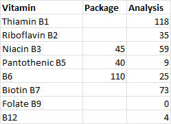
I reached out to Sari Food to ask if their package listed nutritional values for all B vitamins, or if some were omitted.  They confirmed that some were omitted and provided me with a new nutritional analysis that differed significantly from the nutrition reported on the package.  

The new analysis reported 7 B vitamins, compared to the package that only lists 3.  Their analysis showed significant amounts of B1 and B7 that were not listed on the package.  Interestingly, the new analysis also differed from the package for the 3 listed on the package.  I think this shows the variability between different batches of the same product. 

% DV of B vitamins for Sari Nutritional Yeast

Revised Figure showing % DV by brand:

These results increased the average % DV of the 7 brands in my sample for B1 and B7, and decreased the % DV for B6.  This now shows that unfortified nutritional yeast are generally good sources of B1, B2, B3, B5 and B7.  B6 appears to be less common, and I'm not confident that the B9 data is accurate - Sari's new analysis still didn't report any Folate.  Unfortified nutritional yeast is not a good source of B12.

Updated with new analysis from Sari Foods.

Fire Frequency in Arizona Ecosystems

 

Introduction

How likely a given area is to encounter wildfire is important for planning and wildfire mitigation. Historic or expected fire return statistics are often cited for ecosystems in Arizona, but I was curious how often wildfire actually burns across different Arizona ecosystems.

Figure 1 Example wildfire polygons around Clints Well, AZ showing overlapping fires from newer (blue, labelled), to older (shades of brown, unlabelled).  Data sources include WFIGS and GeoMAC.

Wildfire Data

I used the WFIGS Interagency Fire Perimeter GIS data, which has good data on wildfires from 2000-2023.  I limited this analysis to USFS land in Arizona.

Out of a total of 11.168 million acres of USFS land in AZ, wildfire has burned 4.8 million cumulative acres in the last 24 years.  This counts areas that burned more than once as additional acres.  It includes natural and human-ignitions, as well as wildfire managed for resource benefit.  

Figure 2 Example WFIGS Interagency Fire Perimeters in AZ

Figure 3 Wildfire acreage over time in AZ.  2011 was the Wallow fire.

Vegetation Types

To evaluate wildfire probabilities in Arizona ecosystems, I looked at the 15 most common ecosystem types, as defined by the USFS Ecosystem Response Unit (ERU) vegetation type GIS layer.  Together, these 15 ecosystems account for 9.1 million out of the 11.1 million acres of USFS land in Arizona.

Figure 6 Example ERU polygons showing aspen (pink) and mixed conifer around the San Franscisco Peaks, AZ.

To calculate the percent of each ERU burned per year, I divided total acres burned by total acres of ERU and divided that by 24 years.   Spruce-Fire forest and Mixed Conifer is most likely to burn, whereas Mixed Conifer with Aspen is least likely.  Ponderosa pine ecosystems rank in the middle, at around 3% chance. 

This analysis counts acres more than once if they burned more than once in the 24 year time period.  For example, Spruce Fir Forest ERU has more acres of wildfire than there are total acres of ERU.  This does not mean that every acre burned, but some acres burned more than once.   

ERU	ERU Acres	Wildfire Acres	% burned in 24 years	% burned per year
Ponderosa Pine Forest	1,966,603	1,431,424	72.79%	3.03%
PJ Woodland	1,175,545	208,685	17.75%	0.74%
PJ Evergreen Shrub	1,136,221	311,254	27.39%	1.14%
Mojave-Sonoran Desert Scrub	779,939	386,363	49.54%	2.06%
Semi-Desert Grassland	730,015	300,189	41.12%	1.71%
Interior Chaparral	713,754	533,678	74.77%	3.12%
Juniper Grass	539,830	299,074	55.40%	2.31%
Colorado Plateau / Great Basin Grassland	367,114	41,812	11.39%	0.47%
Ponderosa Pine – Evergreen Oak	362,838	238,365	65.69%	2.74%
Madrean Pinyon-Oak Woodland	354,836	92,160	25.97%	1.08%
Mixed Conifer - Frequent Fire	349,006	304,104	87.13%	3.63%
Mixed Conifer w/ Aspen	242,169	9,782	4.04%	0.17%
Montane / Subalpine Grassland	157,163	92,461	58.83%	2.45%
Spruce-Fir Forest	112,827	124,593	110.43%	4.60%
PJ Grass	96,016	8,995	9.37%	0.39%
Madrean Encinal Woodland	93,939	23,092	24.58%	1.02%

Figure 7 ERU acres, wildfire acres, percent burned in 24 years, and percent burned per year.  Table ranked from most to least common ERU.

Wildfire Return Interval

Fire return interval is the average length of time until fire returns at a given point in the landscape.  The chance that any given acre burns depends on a large number of complex factors, including when it last burned, the topography, fuel reduction treatments, proximity to WUI and/or human use.  Still, percent burned per year in the table above (Wildfire/Year, W) can be used to calculate expected return intervals of fire, all else being equal.

Calculations – Fire per Year

To calculate expected return intervals, first calculate the probability (P) that fire will not occur in a given span of time (X).

P = (1-W)^X

For example, for Ponderosa Pine Forest over 10 years:

P = (1-0.0303)^10

P = (0.9697)^10

P = 73.5% chance that fire will not occur, or 26.5% chance that fire will occur in 10 years.

20 years:

(0.9697)^20=54% chance that fire will not occur, or 46% chance that fire will occur.

 

Figure 8 Cumulative probability of wildfire in AZ Ponderosa Pine ERU

Calculations – Fire Return Interval

If we determine a Probability, but need to know the span of time until fire occurs, we can solve for X:

P = (1-W)^X

P = log x / log (1-W)

For example, if we determine "expected return interval" to be the length of time necessary for 50% chance of fire:

 0.5  = (0.9697)^X

X = log (0.5) / log (0.9697)

X = 22 years until there is a 50% chance of fire in Ponderosa Pine Forest.

However, if we interpret "expected return interval" to be the length of time necessary for 90% chance of fire:

0.1  = (0.9697)^x

X = log (0.1) / log (0.9697)

X = 75 years until there is a 90% chance of fire in Ponderosa Pine Forest.

Over time, the probability approaches, but never actually reaches, 100% that a wildfire will occur:

Figure 9 Cumulative Probability of Fire in Ponderosa Pine ERU

Conclusion

The length of time until fire returns at a given point in the landscape depends on how certain we want to be of the chance of fire.  If we want to be very certain (90% probability), then we would expect to wait 75 years on average.  If we are OK taking the flip of a coin (50% probability), than we would expect fire to return at any given point in 22 years.  If we are risk adverse, and can only tolerate a 10% chance of fire visiting our chosen point, we should expect fire every 3.5 years, on average.