My Attempt to Map a Historic Itinerary

Historic newspapers can be illuminating but also frustrating.  A case in point is the series of articles in the 1864 Arizona Miner detailing "Woolsey's Expedition" in March and April of that year.  

I hoped to deduce some of the actual places visited by the expedition, but the details given were confusing, contradictory, and ultimately insufficient to definitively map where the events took place.  I wonder how many modern newspaper stories, when subject to the same analysis, would fall short?

I analyzed Henry Clifton's account from the May 11, 1864 issue.  The first step was to break the narrative into a numbered itinerary.  I underlined what I thought would be helpful clues, and bolded descriptions I thought would be interesting to compare against present day conditions:

My next step was to try to map the itinerary points on a modern day map.  I added two additionally pieces of information to the text.  First, I looked up that sunrise and sunset were at 6:20am and 6:50pm, respectively. This helps fill in the times for each stop.  Then I filled in the mileage between each stop.  In the table that follows, question marks indicate uncertainty.  The start and stop points correspond to the itinerary above.

In some cases Clifton gives the mileage, and in some cases the stops can be determined so the mileage can be measured, but in many cases he does not give the mileage.  However, based on the travel and rest times I tried to estimate the mileage.  This can also be constrained by the possible stop locations.  For example, when they stop at a creek or a canyon, there are only so many choices for where that could be.  

This map shows their possible itinerary from Woolsey's ranch to the Apache Rancheria on "Squaw Creek".  Tent icons are campsites and hiking figures are other stops.  

Overview map showing likely itinerary points.

Waypoint #4 makes sense if they followed the drainage downstream from "Cottonwood Spring" SE to the next main drainage that could be described as "east fork of the Aqua Fria".  This fork is now known as Ash Creek.  The "Ash Creek" they named at stop #5 is most likely the next major creek to the SE, which is now known as Little Ash Creek.

My best guesses for stop #4 and stop #5.

Many mysteries remain.  First, they claim to do a lot of hiking at night, but this is extremely rough terrain that would be difficult to navigate by night.  According to the US Naval Observatory historical moon phase calculator, this expedition occurred during the waning last quarter of the moon, so they would not have had much light from the moon.  I don't know what kind of lanterns they had, but they don't describe much difficulty traveling at night, other than a description that they had to "descend carefully" to a creek for stop #7.

At stop #6, which occurred sometime after 10 PM on the night of March 31st, Clifton reports finding species of the garlic family on a ridge.  These small plants seem like they would have been difficult to notice by lantern light.  Interestingly, there are only two species of garlic/onions that grow in this area in the spring now.  One, is Crowpoison, which as the name suggests is toxic.  The other is Largeflower onion, which is not common.  

Second, was the Apache Rancheria at modern Squaw Creek or some other location?  It would make sense that their place name stuck, but Squaw Creek is not exactly a unique name so it is possible that other locations have the same name.  Interestingly these creeks that form the southeast boundary of Perry Mesa have been recently renamed Ledni Lii Creek, Gosga Creek, Liya Draw, Che Yagoodiguhn Creek, etc.  I can't find any information about when they were renamed or what the new names mean.

Based on their travel that night from 10 PM until 9 AM and their progress on other legs of the journey, I estimated that they traveled about 10 miles to get there.  However, (for reasons discussed below) I think the site of the Rancheria must have been just upstream of the confluence of Gosga creek and Ilya Draw (AKA North Squaw Creek and Squaw Creek), and this would put them less than 7 miles from camp.  After attacking the Rancheria they managed to get back to camp in less time, so it is possible that they were less than 10 miles from camp.   

Possible site of the Ranchera, upstream of the confluence of Gosga creek and Ilya Draw (AKA North Squaw Creek and Squaw Creek)

In the description of the battle, Clifton states that Company C was west of Company B.  Company B "was in the canon below the rancheria" and chased the Indians up the canyon to where company C was.  Since almost all of the canyons in this part of Arizona run from NE to SW, I had a lot of trouble finding a location where "up canyon" was some westerly.  

Conclusion

Through this exercise of interpreting and attempting to map a historical itinerary, I've come to realize the difficulty of matching newspaper accounts to specific locations.  Without an extremely explicit travelogue, creating a location-based itinerary is either impossible or unreliable.  There were several times when I was ready to give up, but through persevering, rereading the account, and staring at the map I've at least been able to convince myself that some of these locations are approximately correct.  I hope to visit some of these areas in the coming months to retrace the route and add additional information.  

Notes

Note: #PrescottAZHistory blog has an account of Woolsey's expedition that is more of a summary and less of a GIS analysis.  

Note 2: Woolsey organized several expeditions, including a second one in June of 1864 that traversed a much larger area.

Wildlife Trends in Arizona: 150 Years of Winner and Losers

 Arizona’s wildlife history is an example of a timeline that occurred in many developing landscapes: an era of exploitation and eradication (1800s–1950s) followed by an era of restoration and management (1980s–present). 

However, there are some factors that were unique to the United States that led to distinct trends in wildlife populations when compared to those same species across the border in Mexico.

The following summary of research (Part 1) lists 16 Arizona species that were extirpated or greatly reduced and whether they have recovered.  Part 2 looks at 10 species that occur in both Arizona and Mexico and why their populations followed different trends.

This research illuminates the current state of wildlife and ecosystems in Arizona and helps explain the factors that got us here.

Part 1: Arizona vs. Wildlife

The following summary organizes species into groups based on their population trajectories: the “Great Returns” that were extirpated but have been successfully reintroduced, the “Survivors” that have been greatly reduced but still persist, and the “Lost Causes” that were extirpated but have not been successfully reintroduced. 

I. The "Great Returns": Extirpated & Successfully Reintroduced

These species were completely removed from the state but have been restored, often using proxy subspecies or captive breeding.

Rocky Mtn Elk

Extirpation Date/Cause: 1900: The native Merriam’s subspecies was hunted to extinction for meat and teeth.

Reintroduction Date/Area: 1913–1928: Rocky Mtn elk from Yellowstone were released near Winslow, Alpine, & Kingman.

Key Trend/Notes: Ecological Substitution: A proxy subspecies filled the empty niche, expanding rapidly due to lack of competition.

Mexican Gray Wolf

Extirpation Date/Cause: 1970: Eradicated by federal predator control programs (poison/traps) to protect livestock.

Reintroduction Date/Area: 1998: Captive-bred wolves released in the Blue Range Primitive Area.

Key Trend/Notes: Predator Tolerance: Success is biologically high but socially controversial; relies on ongoing conflict management.

 

California Condor

Extirpation Date/Cause: 1924: Vanished due to lead poisoning (bullets in carrion) and shooting.

Reintroduction Date/Area: 1996: Released at Vermilion Cliffs.

Key Trend/Notes: Intensive Care: Survival relies on active management (chelation therapy for lead) rather than self-sufficiency.

River Otter

Extirpation Date/Cause: 1950s: The native Sonora subspecies was  trapped out for fur.

Reintroduction Date/Area: 1981–1983:  Louisiana subspecies released in the Verde River.

Key Trend/Notes: Another Proxy: Like the elk, a non-native subspecies was used to successfully fill the vacant ecological role.

Black-footed Ferret

Extirpation Date/Cause: 1960s: Poisoning of their food source (prairie dogs) led to total extirpation.

Reintroduction Date/Area: 1996: Reintroduced in Aubrey Valley (Seligman).

Key Trend/Notes: Disease Barrier: Success is limited by sylvatic plague; requires dusting burrows and vaccines to persist.

Apache Trout

Extirpation Date/Cause: Mid-1900s: Hybridization with non-native rainbow trout and habitat loss.

Reintroduction Date/Area: 1955–Present: White Mtns (managed by White Mountain Apache Tribe & AZGFD).

Key Trend/Notes: The First Win: Became the first sportfish in history to be delisted from the Endangered Species Act (2024).

 

II. The "Survivors": Reduced but Persisted

These species were decimated by unregulated market hunting or predator control but survived in rugged refugia (escape terrain).

Desert Bighorn

Historic Low Point: Early 1900s: Reduced by diseases from domestic sheep and market hunting.

Survival Factor: Terrain: Survived in the most inaccessible desert peaks (Grand Canyon, Kofa).

Current Status: Translocated: Populations are moved to historic ranges (e.g., Santa Catalinas, Virgin River) to ensure genetic diversity.

 

Mountain Lion

Historic Low Point: 1960s: Bountied as "vermin" until 1970.

Survival Factor: Elusiveness: Solitary nature and rough terrain made total eradication impossible.

Current Status: Stable: Managed as a big game species; populations are robust statewide.

Beaver

Historic Low Point: 1890s: Trapped out of major rivers (San Pedro, Santa Cruz).

Survival Factor: Cryptic Behavior: Survived in deep canyons (Verde/Black River) by using bank burrows instead of lodges.

Current Status: Recovering: Reintroduced to the San Pedro (1999); used today for watershed restoration.

Pronghorn

Historic Low Point: 1920s: Fences cut off migration; market hunting reduced herds.

Survival Factor: Open Space: Remnant herds survived in vast private ranchlands (Babbitt Ranches).

Current Status: Managed: Sensitive to habitat fragmentation; relies on modifying fences for movement.

Gunnison’s Prairie Dog

Historic Low Point: 1930s: Poisoned across vast areas.

Survival Factor: Remote Refugia: Survived in the high-elevation Aubrey Valley; resistant to plague.

Current Status: Keystone: Their persistence allowed the Black-footed Ferret reintroduction to happen.

 

III. The "Lost Causes": Extirpated & Failed (or Struggling) Reintroductions

Complex social behaviors or specific habitat needs made simple reintroduction impossible.

Thick-billed Parrot

Extirpation Cause: 1938: Shooting/Poaching.

Reintroduction Outcome: Failed (1986–93): Chiricahua Mtns.

Why It Failed: Cultural Knowledge: Captive birds lacked flock wisdom to avoid hawks and find food.

Masked Bobwhite Quail

Extirpation Cause: 1900: Cattle overgrazing destroyed tallgrass cover.

Reintroduction Outcome: Struggling (1937–Present): Buenos Aires NWR.

Why It Failed: Habitat Specificity: Reintroduced birds often die due to lack of specific cover and predation; almost entirely reliant on captive releases.

Gila Topminnow

Extirpation Cause: 1940s: Invasive Mosquitofish.

Reintroduction Outcome: Mixed/Struggling: Multiple failures in the 80s/90s.

Why It Failed: Invasive Barrier: Cannot survive where aggressive non-native fish are present.

Jaguar

Extirpation Cause: 1963: Killed as predator.

Reintroduction Outcome: Natural Transients Only: No formal reintroduction.

Why It Failed: Political/Social: Only solitary males currently cross from Mexico; no breeding population exists.

Grizzly Bear

Extirpation Cause: 1936: Killed as predator.

Reintroduction Outcome: Permanently Extirpated.

Why It Failed: Social Tolerance: Requires vast, roadless wilderness that no longer exists in AZ; no plans to reintroduce.

 

Unifying Trends in Arizona Wildlife History:

The Predator Paradox:

Predators (wolves, grizzly bears and black bears, jaguars, lions) were targeted by federal policy for eradication to protect livestock.  Only the cryptic/solitary ones (lions, bears in rough terrain) survived. Reintroducing social predators (wolves) has been biologically successful but socially difficult.

The Proxy Solution:

When a native subspecies was completely lost (Merriam's Elk, Sonora Otter), biologists successfully substituted a close relative (Rocky Mtn Elk, Louisiana Otter).  These ecological substitutes often thrived because the niche was wide open and they were generalists.

The Behavioral Barrier:

Reintroductions of intelligent, social animals (Thick-billed Parrot) or habitat specialists (Masked Bobwhite) often fail.  Hard releases (letting animals go) work for generalists like elk but fail for species that require learned behavior or specific micro-habitats.

Part 2: Arizona vs. Mexico

This analysis breaks down Arizona’s extirpated and reduced species by comparing them to their source populations in other U.S. states and their often-distinct fates across the border in Mexico.

The overarching trend reveals a paradox: while the U.S. effectively managed game species (elk, sheep) through public land regulation, Mexico’s private land system (ranchos) inadvertently served as the final lifeboat for nongame species (wolves, prairie dogs, parrots) that were systematically eradicated in the U.S.

Successful Reintroductions: The Game Bias

The species that succeeded in Arizona were often abundant elsewhere in the U.S. but had been wiped out or severely reduced in Mexico.

Rocky Mtn. Elk

Status in Other U.S. States: Thriving: Millions exist across the Rockies (CO, MT, ID).

Status in Mexico: Extirpated / Rare: Native Merriam’s were also lost in Mexico. Small, private herds of Rocky Mtn. elk exist now on high-fence ranches in Coahuila/Sonora.

Accounting for the Difference: Public Land Management: The U.S. model of public land hunting funded the massive translocation efforts. Mexico lacked the public land base or agency funding to replicate this scale of reintroduction.

River Otter

Status in Other U.S. States: Secure: Abundant in the Mississippi Delta and Pacific Northwest.

Status in Mexico: Critical / Extirpated: The native Sonora otter is likely extinct in the Colorado River Delta due to the complete drying of the river before it reaches the sea.

Accounting for the Difference: Water Policy: Arizona’s otters survive in protected flows (Verde/Salt). In Mexico, the water is siphoned off for agriculture before it can support otter habitat.

Mexican Gray Wolf

Status in Other U.S. States: Extirpated: Historically ranged into NM/TX (now reintroduced there).

Status in Mexico: Reintroduced (Struggling): Mexico began releasing wolves in the Sierra Madre in 2011. The population is smaller and more fragile than the AZ/NM population.

Accounting for the Difference: Prey Base: In Arizona, wolves rely on abundant elk. In Mexico, elk are absent and deer are scarcer, forcing wolves to target livestock, leading to immediate conflict with ranchers.

Reduced/Survivors: The Refugia Divide

Species that held on in Arizona often did so in rugged terrain, while in Mexico, their fate depended heavily on the stewardship of individual landowners.

Desert Bighorn

Status in Other U.S. States: Stable: NV, CA, and UT have strong, managed herds.

Status in Mexico: Stable / Commercialized: In Sonora and Baja, bighorn are a high-value commodity. Private ranchers protect them aggressively to sell high dollar hunting tags ($50k+).

Accounting for the Difference: Economic Incentive: In the U.S., bighorn are protected by state agencies as a public trust. In Mexico, they survived because they became a private asset worth protecting from poachers.

Pronghorn

Status in Other U.S. States: Secure: WY and MT have massive herds.

Status in Mexico: Endangered (Sonoran Subspecies): The Sonoran Pronghorn (El Pinacate) is critically endangered.

Accounting for the Difference: Barriers: The U.S. herds had open range. The Mexican herds were hemmed in by highways (Hwy 2) and border fencing, severing their ability to find water during droughts.

Beaver

Status in Other U.S. States: Abundant:  r egained range across the West.

Status in Mexico: Recovering (Delta): The Colorado River Delta saw a miraculous, short-term return of beavers following the "Pulse Flow" (Minute 319) water release in 2014.

Accounting for the Difference: Resilience: Beavers in Mexico proved they are waiting in the wings; they only lack the water, whereas U.S. populations had consistent flows in mountain refugia.

Failed/Struggling: The Mexican Lifeboat

Species that failed in Arizona (often due to poisoning or habitat loss) survived in Mexico, which served as the last stronghold.

Masked Bobwhite

Status in Other U.S. States: Extirpated: Only exists in captivity/refuge.

Status in Mexico: Critical / Persistent: Small wild populations were rediscovered on private ranches in Sonora (e.g., Rancho Carrizo) in the late 20th century.

Accounting for the Difference: Grazing Intensity: While U.S. ranchers switched to exotic grasses (Lovegrass), some remote Sonoran ranches maintained native vegetation due to isolation and traditional (lower intensity) grazing practices.

Thick-billed Parrot

Status in Other U.S. States: Extirpated: No wild flocks in the U.S.

Status in Mexico: Endangered / Extant: ~2,000 birds breed in the Sierra Madre Occidental (Chihuahua/Durango).

Accounting for the Difference: Old Growth Timber: Arizona logged its sky island nesting snags by the 1930s. The remote Sierra Madre retained old-growth forests longer (though these are now threatened by logging).

Jaguar

Status in Other U.S. States: Extirpated: (Breeding populations).

Status in Mexico: Vulnerable / Breeding: A reproducing population exists in Sonora (Northern Jaguar Reserve), only ~120 miles south of the border.

Accounting for the Difference: Road Density: Arizona is crisscrossed by paved roads and development. The Sonoran habitat is more rugged, roadless, and largely privately owned, reducing human-cat interaction.

Black-tailed Prairie Dog

Status in Other U.S. States: Extirpated: Widespread poisoning campaigns.

Status in Mexico: Thriving (Janos): The Janos Biosphere Reserve in Chihuahua holds one of the largest prairie dog complexes in North America.

Accounting for the Difference: Benign Neglect: The U.S. government funded industrial-scale poisoning. The Mexican government lacked the funds for such programs, inadvertently allowing the massive colonies to survive until conservationists bought the land.

Summary of Differences

The Industrial Efficiency of Extirpation

Arizona’s extirpations were often more thorough than Mexico’s because the U.S. had the resources to be efficient. Government-sponsored predator control (wolves/jaguars) and poisoning (prairie dogs) were well-funded industrial operations in Arizona. Mexico, lacking these centralized resources, allowed "pest" species to survive simply through "benign neglect."

Public vs. Private Conservation

Arizona: Success relies on public land management (US Forest Service/BLM). This is great for generalists like elk but hard for specialists that need specific micro-habitats.

Mexico: Survival has relied on private land isolation. Remote ranches in the Sierra Madre acted as unintended nature preserves because they were too difficult to log or develop.

The Elk Gap

The single biggest ecological difference today is elk. Arizona replaced its lost native elk with a massive, successful herd of Rocky Mountain elk. Mexico never did. This means Arizona has a massive prey base for wolves and lions that Mexico lacks, creating a "food imbalance" at the border that complicates predator recovery in the south.

 

Desert People Without Water

I recently visited the ruins at Honanki and Palatki.  These are prehistoric settlements built into the red rock cliffs near Sedona, AZ.  Today, the people who built these dwellings are called "Sinagua", which comes from Spanish for "without water".  But everyone needs water, right?  I wondered where these people got drinking water.

I looked for springs around Honanki and Palatki and didn't find any.  That's weird!

Zoom in to see locations of Honanki (H) and Palatki (P) in relation to USGS-mapped springs (blue) and NAU-mapped springs (green).

Although springs have dried up in recent times, the USGS spring data was mapped in the late 1800s / early 1900s when many more springs were flowing.  It looks like the geology of the Sedona Red Rock cliffs just don't produce springs.  So even if the location of springs was different 800 years ago, it would be surprising if there were springs in the cliffs where these people lived.

The closest mapped spring (blue dot = unconfirmed water source) is 1.5 and 2.7 miles away, respectively, but there is no evidence of water in the aerial imagery.  The next closest (green dot = confirmed water source) is 4.7 and 3 miles away, respectively.   Neither Palatki nor Honanki is even built in one of the larger drainages that might flow more often/longer; the drainages that feed their valleys are quite short.  

I don't think these settlements had access to aboveground water throughout the year unless they dug wells or used cisterns to store water.

These and other prehistoric communities in the desert Southwest often built cliff dwellings high above canyon floors, far from surface water sources.  Archaeologists believe these people collected runoff during rainstorms using check dams and seeps, and stored water in cisterns or ceramic containers for later use.

Across the prehistoric Southwest, populations used ingenious methods to exploit scarce water:

• Rock overhangs and cisterns captured and stored rainwater.
• Seasonal mobility allowed families to occupy dry sites part of the year.
• Terraced fields, check dams, and soil-retention walls conserved moisture for crops.
• Small permanent settlements clustered near ephemeral water sources, such as seeps and seasonal pools.

In conclusion, while many large settlements in the prehistoric Southwest were built near springs or rivers, groups like the Anasazi, Sinagua, and others developed highly effective ways to survive in water-scarce environments through dry-land agriculture, runoff collection, and strategic mobility.

Tortoise Population Zone Trends

Continuing my analysis of iNat tortoise and reptile data, I looked at whether the observed changes in proportion of reptile species encountered was different in urban and urbanizing zones.  I hypothesized that the continuing expansion of large cities in tortoise habitat could be contributing to their decline.

Methods

I downloaded iNat data for AZ reptile species and mapped the points in GIS. I only looked at full species instead of including named subspecies as I had in my previous analysis. Based on that previous analysis, it seemed possible that changes in subspecies identification could be accounting for some of the observed changes and I wanted to remove that potential source of bias.

I then subjectively defined polygons around the large urban zones of Phoenix and Tucson and used the Identify tool to add Phoenix and Tucson labels to all points within those areas.  Note that although the study area includes other towns in Arizona (such as Prescott and Flagstaff) I did not choose to define those areas as "urban". 

Phoenix urban zone.  220 total tortoise observations.

Tucson urban zone:  795 observations.

I also considered whether geopoint accuracy would impact the results, so I conducted the following analysis including and excluding points with no or low (greater than 1000m) accuracy.  However, because I did not see a difference I will simply present results for all data points (i.e. no geopoint accuracy exclusion).

Results: Urban Zones

The majority of tortoise observations are from urban zones, especially Tucson.

It is not possible to determine if more tortoises live around Phoenix and Tucson compared to remote areas; iNat data collection is opportunistic, so places where people live are more heavily sampled than remote areas.  This result is an important caveat to my previous results: iNat observation trends are most representative of urban zones and any observed changes do not necessarily represent changes in all areas of Arizona.

The proportion of tortoise observations has been increasing in urban zones, especially Tucson. From 2013-2025, although there is some noise early on (e.g. 2014) due to low observation counts, the general trend is apparent that Tucson increased from ~45% to ~55% of total observations, while areas outside metro zones decreased from ~40% to ~20%.

This could contradict my hypothesis (that tortoises are declining in areas of urban development), or it could be due to increased observers in urban zones.   

Reptile observations show the same overall trend of increasing observations in urban zones. The proportion of iNat reptile observations for Phoenix increased from 10% to 20%, Tucson increased from 30% to 40%, and non-urban areas decreased from 60% to 45%.

Reptile Observation Trends

I wondered whether the amount of urban versus non-urban observations could explain the changes I observed in reptile species observations.

Updated Reptile Observation Trends

The 26 species of reptiles with more than 1000 observations

There were 26 species of reptiles with more than 1000 observations in the study area.  They ranged from species with 100% urban observations (San Esteban Island Iguana, introduced) to species with 0% urban observations (Plateau Fence lizard).  The colored cells show population change from a 2018 baseline.  Look for areas of red-green or green-red, because those indicate consistent trends from 2013-2025.  Red for both indicate 2018 was a high point.  Green for both indicate 2018 was a low point.  

I then plotted % change against proportion of non-urban observations to look for trends and outliers.

First graph: The point at 100% non-urban and 50% change is Plateau Fence lizard, which is very common in Prescott and Flagstaff, maybe that area should be an urban zone.  The point above 200% change is sidewinder, maybe someone was studying them back in the day?

2nd graph.  The point at 0% nonurban and 180% change is the iguana, introduced in Tucson.

Conclusion

Urban areas do not have a consistent negative or positive impact on reptile observation trends. It would be interesting to look at observation trends of individual species in each zone, but most species do not have enough observations for a meaningful statistical analysis.

At this point I can conclude that the large and increasing share of iNat observations from urban areas definitely affects the analysis of reptile observation trends, but I have not been able to identify a consistent bias that this would introduce into my overall analysis.

Sonoran Desert Tortoise Population Status

 Abstract

Population trend data for species under consideration for federal protection is often limited. This study evaluated Sonoran desert tortoise (Gopherus morafkai) population trends in Arizona using iNaturalist citizen science data. We analyzed 1,402 research-grade tortoise observations and normalized them against total observations in the area to account for sampling bias. While both tortoise observations and total observations increased since the early 2010s, the ratio of tortoise to total observations declined consistently from 0.12% to 0.08% between 2017-2025. This decreasing ratio suggests either shifting observer preferences or declining tortoise encounter rates, potentially indicating population decline. These results provide concerning evidence of negative population trends for this species of conservation concern and demonstrate the utility of citizen science data for monitoring species lacking formal survey programs.

Introduction

Sonoran desert tortoise (Gopherus morafkai) live in the Sonoran desert of Arizona and northern Mexico.  A closely related species in California and Nevada, the Mojave desert tortoise (Gopherus agassizii), is Federally protected as a Threatened species under the Endangered Species Act (ESA).  The Sonoran desert tortoise is listed by AZ as a Species of Greatest Conservation Need (SGCN) and was proposed for protection under the ESA but determined "Not Warranted" in 2022.  On June 4, 2025 wildlife groups filed suit in federal court challenging that determination.  

It is difficult to find current population trend data for species that may warrant listing under the ESA, so I attempted to do so using publicly available iNaturalist data.  iNaturalist is a public repository of photographic observations of species.  

Methods

I filtered iNat for Research Grade observation of Sonoran desert tortoises in AZ and found 1,402 observations. I considered limiting the analysis to only live tortoises, but eventually decided to use all research grade observations due to the difficulty filtering. Only ~3% (44 observations) were annotated as dead , and only ~1% (12 observations) were annotated as scat.  

I created an Area of Interest (AOI) bounding box around the tortoise data to search for total RG observations.  There were a total of 1.2 million RG observations in the Sonoran desert of southern AZ.

RG tortoise observations in AZ with bounding box showing AOI.  

More tortoises are observed in places where there are more people to observe them.  Because iNat data is based on opportunitistic data collection, it is liable to biases based on where people live as well as how many people use iNat.  To attempt to correct for this, trend analyses can normalize the count of tortoise observations as a ratio of total observations in the AOI.


Data

Data table of AOI with Total RG Observations, Total Observations, RG:Total Observations Ratio, RG Tortoise Observations, and RG Tortoise: RG Total observations.

Results

Total RG observations in the AZ Sonoran desert have been increasingly consistently since the early 2010s.

Count of total RG observations in the AOI per year.

Tortoise observations have increased since 2013, with some notable dips in 2020 and 2023. It is possible that these dips are due to weather-related impacts to tortoise population, but they could also be due to differences in number of observations.  

Count of tortoise observations per year.

By comparing tortoise observations to total observations, a normalized ratio can be derived. This ratio decreases over time. There is a step change decrease in 2017, which could be a real population decrease or could be due to the huge increase in popularity of iNat in 2017.  However, even if only looking at 2017 -2025, there is still a long term decrease in the ratio of tortoise observations, from around 0.12% to 0.08% of total observations. 

Ratio of tortoise observations to RG observations. 

Discussion

The decreasing ratio of tortoise observations indicates that either people are trending to preferentially observe other species more than tortoises, or that tortoises are making up a smaller percentage of the animals people encounter.  

Despite limitations of citizen science data, these results provide concerning evidence of negative population trends for this species of conservation concern and highlight the utility of iNaturalist data for monitoring species that lack formal survey programs.

The Knife Edge of Spring

"To what purpose, April, do you return again?

Beauty is not enough.

You can no longer quiet me with the redness

Of little leaves opening stickily."

-from Spring by Edna St. Vincent Millay

In AZ, the spring green up of grasses and trees makes use of a narrow window of time between declining winter moisture and increasing summer heat.  Our redbud trees blooms for three or four days (this year, from April 26-29), the lilac bushes hardly last much longer, and the spring green up of weedy lawns is over by the end of May.  June is the dry season in Arizona.  June is when spring dies.

The knife edge of spring in Arizona can be seen in the biomass production.  For example, the Rangeland Analysis Platform shows that peak spring growth in Dugas, AZ in 2020 lasted approximately 3 weeks, from 4/1 to Earth Day 4/22.  By May, the growth of the annual green up was already in freefall.  More examples can be seen in this previous blog post using RAP to investigate biomass production variability from year to year.  

Phenology Mapping

The National Phenology Network's Visualization Tool can be used to follow the spring green up via Accumulated Growing Degree Days (AGDD), which work by adding up all of the days and temperatures above some minimum threshold for growth, usually 32 F for cool season plants (winter annuals, cool season grasses, willows and cottonwoods and other early spring plants) or 50 F for warm season plants (mesquite, acacia, and other warm season trees like Chilopsis, walnut, and warm season grasses and forbs).

AGDD Details

A "growing degree day" (GDD) is calculated by subtracting the threshold temperature (T) from the average temperature for each day when the minimum temperature is above the threshold temperature of 32 or 50 degrees. 

Average T = (Maximum T - Minimum T)  / 2

GDD = Average T - Threshold T

 Accumulated growing degree days (AGDD) simply adds up all of the GDD since the beginning of the year.

AGDD = GDD (January 1) + GDD (January 2) + … + GDD (yesterday)

To use the NPN Visualization Tool for AGDD, choose Map>Base Layer>Category: Daily temperature accumulations>Layer:Current Day.

AGDD Example - 32 F

The figure below shows AGDD around Prescott, AZ from a threshold temperature of 32 as 5/2/24.  Most of the map shows AGDD of about 2,000; since there have been about 120 days since the beginning of the year, that works out to an average daily temperature of 48 degrees F (2,000/120 + 32 =  48).  Of course, some areas have been warmer than that and some have been cooler:  

Phenology AGDD from 32 F 

1,600 - cottonwoods leafed out (Prescott)

1,800 - still winter grasses not green (Kirkland junction)

2,200 -  annual grasses very green, early spring wildflowers blooming (Dugas)

2,245 - mesquite not leafed out yet, annual grasses still somewhat green (Yava)

2,500 - mesquite leafed out, annual grasses brown (Date)

2,800 mesquite flowering (Congress)

AGDD Example 50 F

Or maybe a 50 degree threshold better shows mesquite and grass green up? The average daily temperatures, of course, are the same, but the different threshold yields much lower AGDDs, mostly in the low 100's.  On this map, light green area are grasses already brown and mesquite leafed out, green areas actually are green fields of annual grasses, whereas white and blue are areas where willows, cottonwoods, and elms have leafed out, but herbaceous plants are just barely getting started.

Phenology AGDD from 50 F 

240 - oaks turning brown (Kirkland)

350 - mesquite not greened up yet, annual grasses and forbs green (Dugas)

400 - mesquite not leafed out yet, annual grasses still somewhat green (Yava)

550 - mesquite leafed out, annual grasses brown (Date)

800 - mesquite flowering (Congress)

AGDD Anomalies

The examples above of specific phenology AGDD values can be used in conjunction with NPN's Visualization Tool to predict plant growth stage.  Also, it is possible to use NPN's Visualization Tool to highlight geographic areas that may be ahead or behind the usual spring green up using the "Anomaly" visualization.  In the figure below, anomaly from 32 F AGDD, it can be seen that the Kirkland valley, Black Canyon City, and the Verde valley are behind (blue) normal phenology, whereas Prescott valley and especially the area north of Bagdad are ahead (red) normal phenology.  

"Life in itself 

Is nothing,

An empty cup, a flight of uncarpeted stairs.

It is not enough that yearly, down this hill,

April

Comes like an idiot, babbling and strewing flowers."

-from Spring by Edna St. Vincent Millay

Tree Risk - notes

 Notes from Tree Risk Assessment Qualification (TRAQ) class taught by Kevin Eckert for the Arizona Community Tree Council.  October 2022 

About 25 people are killed each year by falling trees in U.S.

Removal should only be an option when mitigations are not sustainable.  We have an ethical obligation to do no harm.  The benefits of trees are important.  

A risk is meaningless without a time frame.

Imminent - if a tear in the tree is weathered, the failure is not Imminent

Probable - failure would likely occur during normal (expected/seasonal) extreme weather.

Possible - failure would likely occur during abnormal (hurricane, tornado, derecho, etc) extreme weather.

Wounds

Thicker sap trees tend to compartmentalize better

If sap is oozing, touch and smell it:

Sticky = ok, its sap

Sour = bacteria

Slimy or foamy = fungus

Wet = just water

Drought

Tree dying from bottom up is over-irrigation

Tree dying from top down is drought (under-irrigation)

Failure

Soil failure vs root failure:  roots in air or roots break and stay in ground

Codominant is not a fault.  

Included bark is a fault because weak area doesn't hold stems.  

Aspect ratio near 1:1 for codom stems is a fault because don't have enough wood to wrap around union.  This is common cause of failure in pines, especially CA fire investigations.

Decay

Worse on compression side and at the base.  Hollow poles are strong. Most stress in tree is around the shell, so sapwood carries most weight, not heartwood (which is more brittle).

Heartwood - least concern

Sapwood - will start seeing tip dieback. 2nd worst.

Root - will also see tip dieback.  Not too bad if not structural; crown dieback will balance root dieback.

Basal - worst.  

Types of Response growth:

Reaction wood from tension/compression

Flexure wood from movement

Wound wood - e.g. lip around wound. More growth shows more stress

Likelihood of failure increases/decreases based on load (e.g. wind exposure) / response growth

Stress

Reproduction is sign of stress in trees (plants):  orchard trees cut to fruit more, but decreases lifespan.

Vigor/health does not always reduce tree failure risk

Adding N can increase leaf area and stem elongation, but that can increase load on stem and if stem doesn't thicken then can increase tree failure risk, even while increasing tree "vigor".  Sometimes reducing growth (ie use growth regulator) can improve mitigations.

Sheer plane: where tension and compression meet

Cracks: transverse (fiber failure) or longitudinal (with the grain)

Age

Old trees: retrenchment = natural process of aging, shortening and widening = more stable

Trees naturally move with wind.  Mass damping shows importance of inner branches and leaves.  Helps tree stems "undulate like snake in the wind".  Sharp bends or lack of inner leaf area can inhibit natural movement.

Construction

New concrete can leach lime/calcium oxate which raises soil pH and can harm some plants if too much

Adventitious branches = "water sprouts" (from topping = non ANSI cuts) = epicormic.  Poor attachments can rip out.

Shigo said:  "don't err on the side of safety….just do it right!"  :: Do the best you can based on your education, training, and experience.  

Arizona Monarchs Visit California and Mexico

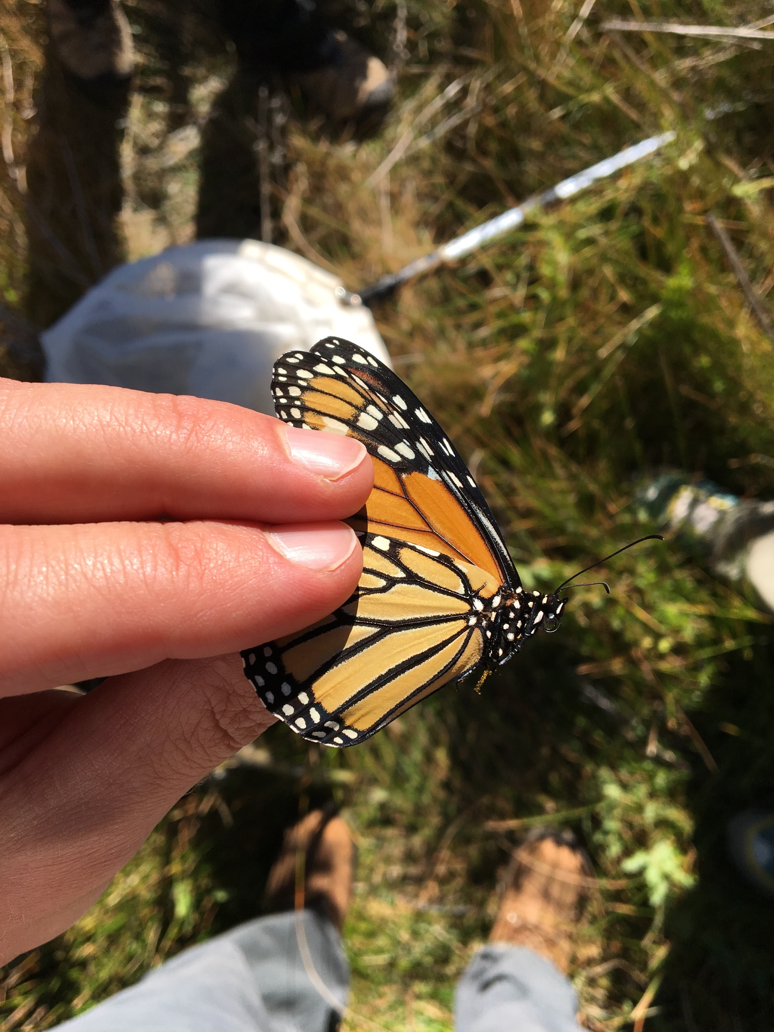
 Five years ago my wife and I joined other local citizen scientists at Willow Lake for an enjoyable afternoon catching and tagging monarch butterflies.  The tags are small stickers with ID numbers.  They  don't impair the butterfly's ability to fly, but they do let us humans track where they fly to!

A monarch in the hand.

 The Southwest Monarch Study group recently updated their map showing the location of recovered tags.  The straight lines indicate starting and ending locations, not necessarily the meandering paths monarchs take to migrate across the landscape. 

Image from Southwest Monarch Study.  

  Over the ensuing years, those tagged butterflies have turned up as far away as the monarch's overwintering grounds in Mexico. Interestingly, they also visit California overwintering sites.  Most monarch populations can be neatly divided into Eastern and Western populations based on where they spend the winter; Eastern go to Mexico and Western go to California.  But it seems AZ monarchs can go to either, which raises the fascinating question: how do they decide where to go?  Is AZ a meeting spot for different populations, and each return to their home wintering sites, or is AZ a melting pot, a single population where individuals decide each year where to overwinter?

Hopefully this citizen science research will help resolve some of the question marks on monarch migration maps.

Monarch migration map from Xerces.

Monarch migration map from Monarch Watch. 

Biodiversity on Prescott National Forest

 How many plant species are there in a geographic area?  Previously, I used iNaturalist to calculate total biodiversity for selected areas.  But this method is just a snapshot of the species currently recorded in iNaturalist.  In some areas, people may have already observed most of the biodiversity, while in other areas there may still be much more to discover.

One way to estimate the total unobserved biodiversity of a geographic area is to look at the timeline of species observations.  If more new species are being observed each year, there are likely still many more species to discover, whereas if the number of new species each year is declining, we may be able to fit a decay function that would predict the total number of species that will ever be observed.

iNaturalist offers a couple of ways to find lists of new species.  As an example, I will use the Prescott National Forest in AZ.

The first method: the API function recent_taxa.

According to this method, there have been 57* new plant species observed on the Prescott National Forest in iNat so far this year.  This is filtered for only research grade observations (quality_grade=research).  There are a lot of new observations by experts that just haven’t been confirmed by other experts. *For some reason this returns the species, genus, and family so to get 57 I subtracted repeated taxa (29) from total new taxa this year (86).

https://jumear.github.io/stirfry/iNatAPIv1_identifications_recent_taxa.html?place_id=130970&taxon_id=47126&hrank=species&order=desc&order_by=created_at&per_page=200&quality_grade=research

The URL code is pretty easy to modify for other places (PNF = 130970) and other taxa (plants = 47126).  Here is more background on API query terms: https://api.inaturalist.org/v1/docs/#!/Identifications/get_identifications_recent_taxa

The second method: download data.

 When searching observations for Prescott National Forest and filtering by plants, iNaturalist returns a page with summary statistics.   This can be downloaded and analyzed in Excel.

https://www.inaturalist.org/observations?place_id=130970&iconic_taxa=Plantae 

 After downloading the data:

1. sort the table from oldest to newest by the observation date column

2. select the whole table

3. use “remove duplicates”, and look for duplicates in only the species name column

The resulting list will show you the first observation of each species.  I then summarized the list by year and created this graph showing the year and number of new plant species recorded in iNaturalist for PNF.  

This method also sometimes returns other taxa than species, so the totals don't quite match between the website, the API, and this method.  Also, this graph is not filtered for only Research Grade observations, but it would look basically the same.  The graph appears to increase over time as more people use iNaturalist to record plant species on Prescott National Forest, up to a peak year in 2020.  Since then the number of new species seems to fall off, although it should be noted that 2021 was a drought year and 2022 isn't over yet.