Fire Frequency in Arizona Ecosystems

 

Introduction

How likely a given area is to encounter wildfire is important for planning and wildfire mitigation. Historic or expected fire return statistics are often cited for ecosystems in Arizona, but I was curious how often wildfire actually burns across different Arizona ecosystems.

Figure 1 Example wildfire polygons around Clints Well, AZ showing overlapping fires from newer (blue, labelled), to older (shades of brown, unlabelled).  Data sources include WFIGS and GeoMAC.

Wildfire Data

I used the WFIGS Interagency Fire Perimeter GIS data, which has good data on wildfires from 2000-2023.  I limited this analysis to USFS land in Arizona.

Out of a total of 11.168 million acres of USFS land in AZ, wildfire has burned 4.8 million cumulative acres in the last 24 years.  This counts areas that burned more than once as additional acres.  It includes natural and human-ignitions, as well as wildfire managed for resource benefit.  

Figure 2 Example WFIGS Interagency Fire Perimeters in AZ

Figure 3 Wildfire acreage over time in AZ.  2011 was the Wallow fire.

Vegetation Types

To evaluate wildfire probabilities in Arizona ecosystems, I looked at the 15 most common ecosystem types, as defined by the USFS Ecosystem Response Unit (ERU) vegetation type GIS layer.  Together, these 15 ecosystems account for 9.1 million out of the 11.1 million acres of USFS land in Arizona.

Figure 6 Example ERU polygons showing aspen (pink) and mixed conifer around the San Franscisco Peaks, AZ.

To calculate the percent of each ERU burned per year, I divided total acres burned by total acres of ERU and divided that by 24 years.   Spruce-Fire forest and Mixed Conifer is most likely to burn, whereas Mixed Conifer with Aspen is least likely.  Ponderosa pine ecosystems rank in the middle, at around 3% chance. 

This analysis counts acres more than once if they burned more than once in the 24 year time period.  For example, Spruce Fir Forest ERU has more acres of wildfire than there are total acres of ERU.  This does not mean that every acre burned, but some acres burned more than once.   

ERU	ERU Acres	Wildfire Acres	% burned in 24 years	% burned per year
Ponderosa Pine Forest	1,966,603	1,431,424	72.79%	3.03%
PJ Woodland	1,175,545	208,685	17.75%	0.74%
PJ Evergreen Shrub	1,136,221	311,254	27.39%	1.14%
Mojave-Sonoran Desert Scrub	779,939	386,363	49.54%	2.06%
Semi-Desert Grassland	730,015	300,189	41.12%	1.71%
Interior Chaparral	713,754	533,678	74.77%	3.12%
Juniper Grass	539,830	299,074	55.40%	2.31%
Colorado Plateau / Great Basin Grassland	367,114	41,812	11.39%	0.47%
Ponderosa Pine – Evergreen Oak	362,838	238,365	65.69%	2.74%
Madrean Pinyon-Oak Woodland	354,836	92,160	25.97%	1.08%
Mixed Conifer - Frequent Fire	349,006	304,104	87.13%	3.63%
Mixed Conifer w/ Aspen	242,169	9,782	4.04%	0.17%
Montane / Subalpine Grassland	157,163	92,461	58.83%	2.45%
Spruce-Fir Forest	112,827	124,593	110.43%	4.60%
PJ Grass	96,016	8,995	9.37%	0.39%
Madrean Encinal Woodland	93,939	23,092	24.58%	1.02%

Figure 7 ERU acres, wildfire acres, percent burned in 24 years, and percent burned per year.  Table ranked from most to least common ERU.

Wildfire Return Interval

Fire return interval is the average length of time until fire returns at a given point in the landscape.  The chance that any given acre burns depends on a large number of complex factors, including when it last burned, the topography, fuel reduction treatments, proximity to WUI and/or human use.  Still, percent burned per year in the table above (Wildfire/Year, W) can be used to calculate expected return intervals of fire, all else being equal.

Calculations – Fire per Year

To calculate expected return intervals, first calculate the probability (P) that fire will not occur in a given span of time (X).

P = (1-W)^X

For example, for Ponderosa Pine Forest over 10 years:

P = (1-0.0303)^10

P = (0.9697)^10

P = 73.5% chance that fire will not occur, or 26.5% chance that fire will occur in 10 years.

20 years:

(0.9697)^20=54% chance that fire will not occur, or 46% chance that fire will occur.

 

Figure 8 Cumulative probability of wildfire in AZ Ponderosa Pine ERU

Calculations – Fire Return Interval

If we determine a Probability, but need to know the span of time until fire occurs, we can solve for X:

P = (1-W)^X

P = log x / log (1-W)

For example, if we determine "expected return interval" to be the length of time necessary for 50% chance of fire:

 0.5  = (0.9697)^X

X = log (0.5) / log (0.9697)

X = 22 years until there is a 50% chance of fire in Ponderosa Pine Forest.

However, if we interpret "expected return interval" to be the length of time necessary for 90% chance of fire:

0.1  = (0.9697)^x

X = log (0.1) / log (0.9697)

X = 75 years until there is a 90% chance of fire in Ponderosa Pine Forest.

Over time, the probability approaches, but never actually reaches, 100% that a wildfire will occur:

Figure 9 Cumulative Probability of Fire in Ponderosa Pine ERU

Conclusion

The length of time until fire returns at a given point in the landscape depends on how certain we want to be of the chance of fire.  If we want to be very certain (90% probability), then we would expect to wait 75 years on average.  If we are OK taking the flip of a coin (50% probability), than we would expect fire to return at any given point in 22 years.  If we are risk adverse, and can only tolerate a 10% chance of fire visiting our chosen point, we should expect fire every 3.5 years, on average.

Best Summary of A New Kind of Science

Wolfram's blog.

Calibrating Bank Full Measurements Using Regional Curves and USGS Stream Guage Data

Bankfull is important to fluvial hydrogeomorphology (HGM) because it often determines the shape of the channel by moving and depositing sediment. Bankfull (BF) is defined as the high water level that recurs every 1 - 2 years, but measuring it in the field involves using multiple indicators in a 'preponderance of evidence' detective-style approach.

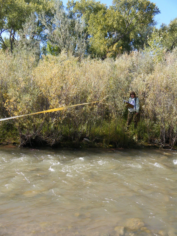
Most plants that cannot tolerate saturated soil conditions for days at a time, like Alders, will not grow below BF, while willows and cottonwood can. Also, the top of point or side bars can indicate the height of BF, but on the Rio Embudo, near Dixon NM, BF indicators were contradictory and hard to find. Is BF just a few centimeters above the base-flow water, or are all the willow below BF?

From Rio Embudo at Dixon, NM Hydrology Analysis

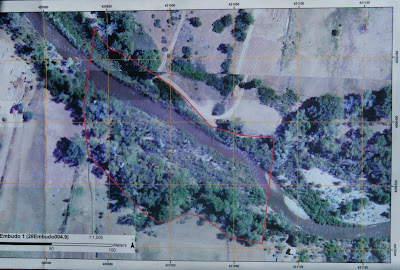
A number of bars and scour features at different heights further compounded the mystery. It was time to seek out other clues. One source of potential indicators was our aerial imagery, which was taken during Spring runoff, 2008:

From Rio Embudo at Dixon, NM Hydrology Analysis

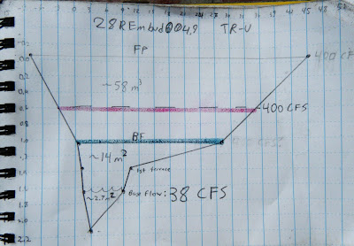
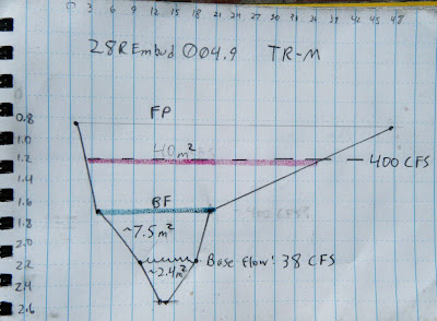
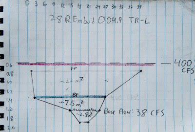
The point bars at bottom right are bisected by a side channel that is several feet above the base level today. That means BF must be at least that high, and would probably inundate most of the willows. Corroborating this, the landowner reports that the willows are indeed flooded almost every year. But exactly how high is BF? To gather more data, we surveyed three channel cross sections, or transects (TR), noting the heights of the major terraces.

TR-Upper

From Rio Embudo at Dixon, NM Hydrology Analysis

TR-Middle

From Rio Embudo at Dixon, NM Hydrology Analysis

Tr-Lower

From Rio Embudo at Dixon, NM Hydrology Analysis

On each of these cross sections we marked where the current base flow water level is, where we think BF is, and where we think Flood Prone (FP) might be. To check these guesses, we correlated those heights with flow data from a USGS gauge just downstream:

From Rio Embudo at Dixon, NM Hydrology Analysis

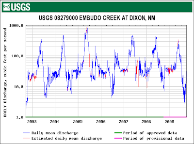
From this graph we could see that the high water level with recurrence every 1 -2 years is about 400 cubic feet per second (CFS). We could also see that the current flow was about 38 CFS. If the Rio Embudo is flowing with 38 CFS today, how high would a BF flow of 400 CFS be?

between the flow today and BF flow. To figure that out we might need to correct for any changes in the velocity (feet/second). Manning's Equation:

shows that velocity V is proportional to a constant, u, inversely proportional to a coefficient of friction, n, varies to the 2/3 power of channel cross-sectional area, R, and to the 1/2 power of slope, S. Since neither slope nor the constant would change, we can discount them and focus on n and R; n will likely increase because the willows will act like a series of giant combs, increasing friction, and R will also obviously have to increase. For example, doubling the height of the water would multiply that term by 1.6. Unfortunately, coefficients of friction need to be experimentally determined, so we can only guess at n. To make things easier, I decided friction would also increase by a factor of 1.6, to exactly cancel out R. In other words, I don't think the velocity would change by much.

So it is a simple matter of geometry to calculate the cross-sectional area that would correspond to 400 CFS on our cross sections (red lines on the cross-sections, above). Without exception, this height is higher than our field-determined BF (green lines on the cross-sections, above) and, at least for TR-L, even higher than our FP height.

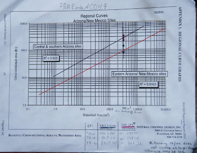
But is this right? Are we getting closer to the truth? To check, we can calibrate our answers for the Rio Embudo against data published by Natural Channel Design on a large number of other Southwestern rivers:

From Rio Embudo at Dixon, NM Hydrology Analysis

I plotted both our field-determined BF cross-sectional area (green points) and the USGS-determined BF cross-sectional area (red points) on the regional curve above. The green points seem to fall on the line for New Mexico, while the red points fall on the Arizona line, corroborating our field measurements and casting doubt on the USGS. However, the watershed above Dixon is very impermeable and could behave more like AZ than NM. I think the true value is probably somewhere in-between the field and USGS values.

This line is probably as close as any to Bankfull:

From Rio Embudo at Dixon, NM Hydrology Analysis

The Day After Tomorrow

The movie "The Day After Tomorrow" is about the end of the world, and, unexpectedly, the cinematography is fairly good. I was surprised by how much I enjoyed seeing Los Angeles destroyed. New York is another matter: NY is destroyed every other weekend at the box office, and I've never lived there anyway, but I have lived near LA and I now believe that every good movie should destroy something important in your life.

Plus, the scientific side of the story was thought-provoking. Catastrophic (saltational) climate change can't be ruled out based on our present state of knowledge. The fossil record isn't precise enough to determine if past climate changes happened in 5, 50, or 500 hundred years. Also, the current level of Co2 is unprecedented for at least the last 400,000 years (the limit of our ice core data) and the rate of increase is likely unique in the entire history of the planet. We simply don't know enough from past experience to accurately anticipate how this is all going to play out.

The IPCC has issued a series of scenarios with likely average temperature increases, but a thorough understanding of the problems inherent in such models calls into question the precision of these averages. The most commonly cited average gives increases of of 2-6C over the next 100 years. But all of the models they currently use are inherently gradualist models (more on this below). One could be a skeptic whether these models are accurate at all, but their (retrograde) prediction of the cooling associated with the Mt. Pinatubo eruption convinced many of their validity. It is edifying to note the maturation of models that originally didn't even take into account atmospheric dust; this is certainly a new science and many problems remain to be solved, particularly the response of vegetation to increased CO2. (CF. McNaughton & Jarvis. Effects of spatial scale on stomatal control of transpiration. Agricultural and Forest Meteorology, 54, 279-301). There is a definite possibility that other, as yet undetermined, variables could play a significant role in future climate change.

But the problem with relying on IPCC averages as outer limits of possible climate changes goes deeper than possible 'out of left field' variables. A recent effort using contemporary day-to-day "matrix" models of weather (e.g. the kind that are used to predict the path of hurricanes) to predict long term climate change yielded slightly higher averages (up to 11C) than the IPCC,. But the most important result was buried in the calculation of these averages. It turns out that the researchers, like many other modelers, ran their simulation thousands of times and only averaged the results that seemed reasonable. A significant proportion of the models "crashed" to negative or positive infinity temperature. Obviously, these results could not be averaged with the simulations that "worked", but they instead point to the instability inherent in these equations.

The climate change models and the way they are interpreted are inherently biased toward gradualist results, but the real danger of climate change is unpredictability. A perfect storm probably won't jump-start a renewed ice age in a manner of days, as in The Day After Tomorrow, but more humble respect for the mysterious potentialities of nature may be wise. The hubris of those who calculate the economic cost of the IPCC predicted change are one example of what can go wrong in a cost-benefit analysis that doesn't factor in the possibility of catastrophes. Attaching specific temperatures to the future climate of the earth is an important undertaking, but it is not a perfect science. Nothing is.

Mathematics and Mileages to my House

The trail to my house, as all trails in the Southwest, is a wash (or vise versa). You go along down the dirt road where the BLM rangers lost my tracks. When the tire ruts have begun to meander individually, separate from one another, you have come to the right spot. Now they split and go around trees that are 50 years old.

They tracks have become trails.


But these trails are no longer monotonic, (one-to-one) i.e. for a given distance from the trailhead there are different, yet equivalent, positions on the trail. In other words there are many trails masquerading as one another.

Suddenly, you are at my camp.

Teaching lesson plans

teaching lesson plans
1) find the center of the triangle
http://en.wikipedia.org/wiki/Incircle



2) alphabet on beyond zebra cyrillic arabic etc

Aspirin, tinnitus, and OAEs

Otoacoustic emissions (or OAEs) are sounds that your ear makes on its own and as a response to environmental sounds. It appears to be some sort of active resonance or tuning and is different from tinnitus, the ringing sometimes heard in quiet rooms. OAEs provide a non-invasive way of evaluating the health of the ear; OAEs disappear almost immediately upon onset of deafness or death (it was only recently that scientists realized that live ears respond differently from dead ones). Interestingly, aspirin also abolishes OAEs. This is a whole new field of research.

Lesson Plan #1. Relationships: Analogy and Resemblance

Relationships: analogy, resemblance

In education, we teach you what kind of assumptions you can make.
Everyone has seen the kid who sees a bird and then thinks that he can fly.
This is false.
Unless he can generate sufficient lift to overcome gravity. Orbits, bernouli, etc.

Now: correspondence. When are two things equal? Equivalent: right and left hand.
Cardinal number (e.g. 5 or infinity) natural numbers vs. transfinite cardinal numbers
Name an infinite set: the set of all natural numbers
Denumberably infinite set is given a name: aleph-null.
Other examples: all even numbers (show correspondence)
All pairs of natural numbers; [therefore rational fractions]
Arranged diagonally: ((1,1)>(2,1)>(1,2)>(1,3)>(2,2)>(3,1)>(4,1))

Aren’t all infinite sets denumerably infinite then?
No: real numbers
Start simple: between 0 and 1
Make a correspondence: 0.20746….=1
0.16238….=2
0.97126….=3

Until you have a countably infinite list. But now construct a new decimal whose first digit is different from 1, whose second is different from 2, whose third is different from 3, etc. Continue until you have a decimal that is different from the infinite number already given. Obviously you could do this at least 8 other times, and then a new order would suffice to let you do it again, and again, and again…

Thus the set of natural numbers and the set of real numbers are not equivalent
The set of real numbers is called transcendental numbers. It is equivalent both to a line (or any size) and the plane(!), or a space of any dimension.

A new tool for making bigger infinities: The set of all subsets.