Showing posts with label precipitation. Show all posts

Monday, April 13, 2026

"Average" Rainfall in Arizona

 NOAA National Water Prediction Service reports daily, weekly, monthly, seasonal, and yearly accumulated precipitation and the totals can compared to "normal".  Their data access website states that normal precipitation is defined as the 30-year PRISM normal from 1981-2010.  The Parameter-elevation Regressions on Independent Slopes Model (PRISM) climate mapping system developed at Oregon State University are considered the most detailed, highest-equality spatial climate datasets currently available.

But is the average still the same in the 16 years since 2010?

Methods

I downloaded total accumulated precipitation for water years ending September 30 for the last 10 years.  Unfortunately, the files for many of the years were corrupted and I was only able to look at the three years from October 2022-Oct 2025.  

I clipped the rasters to the Southwest US and took the mean for each grid cell.

Results

Over the last three years, some areas of the Southwest have had 50% of normal precipitation, and other areas have had 150% of normal. 

NOAA NWPS % of normal 2023-2025

Color key:


Zooming in to the area around Prescott, Arizona:

NOAA NWPS % of normal 2023-2025

Conclusions

Most of the area around Prescott is between 85-95% of normal (medium orange), confirming the presence of long-term drought.  Areas less than 75% of normal (dark orange/red) include much of the Bradshaw mountains around Prescott, the Dugas area along I-17, the Mogollon Rim - east of Payson and from Sedona to Ash Fork, and the south slopes of the San Francisco mountains around Flagstaff.

However, there are significant areas between 115 and 125% of normal (light green), including some areas above 125% of normal (dark green).  These above-average areas include the Juniper mountains and Upper Verde River, the Santa Maria river near I-93, a bit of Sedona and Schnebly Hill to Mormon Lake, and the north side of the San Francisco mountains. 

This shows how spatially heterogeneous average rainfall can be, and how a simple description of a state as being in drought or not can be misleading. For example, the excellent Drought Aware web app from Esri shows broad swaths of Arizona currently in drought, but my analysis shows that there is likely much more spatial variability.  

Tuesday, July 30, 2024

How to Use Satellites to Find Growing Plants: A Practical and Theoretical Guide


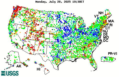
USGS Maximum consecutive dry days, July 2024


Introduction

Knowing where and when plants are green and growing would help botanists and ecologists plan field work and help managers make real-time land management decisions.  There are many potential sources of geospatial data available but it is difficult to know which sources are most useful.

Over the past year I evaluated the accuracy and interpretability of dozens of indicators that could be used to assess current growing conditions.  These websites, maps, and data layers are mainly provided by US Government agencies to help managers respond to natural resource concerns such as rangeland management and drought impacts.

In my opinion, none of the available resources is a perfect fit to find growing plants.  However, understanding how plant growth is related to biophysical constraints can help identify the best available resources.


Plant Growth Theory

Plant growth (Net Primary Productivity, NPP), is proportional to total soil moisture (SM) and Growing Degree Days (GDD) of accumulated Temperature (T) since the start of that plant's growing season.  Soil moisture depends upon accumulated (total and frequency of ) precipitation (P) minus evapotranspiration (ET).  

 NPP = Sum (SM*T)

 SM = Sum (P-ET)

[In the above equations, "equals" is used to mean proportional, or depends upon. ]

The ideal resource for plant growth would be a direct measurement of NPP.  A second option would be measurement of soil moisture and temperature, with a way of combining them to estimate NPP.  A third option would be measurement of precipitation, which could be used to estimate SM. All of these variables can be measured via satellite, but delays make them difficult to use in real time.  Also, there are important details in how they are measured and modelled that make interpretation difficult.  


Details

Plant Growth: satellites can measure NPP via NDVI (Normalized Difference Vegetation Index), but available sources are delayed (DroughtView), low-resolution (GIMMS), weighted toward trees, and contain artefacts early in the growing season.  Existing models of NPP are not well-calibrated (VegDRI), or delayed and not mapped (RAP).

Soil Moisture: satellites can measure SM, but satellite data (SMAP) is not consistently available, may be inaccurate, and only provides a snapshot, not the sum.  Models of SM are not well-calibrated (NASA LIS).

Temperature: sensor networks can measure T and calculate Growing Degree Days (NPN) but aspect and micro variation are often more important than county-level temperatures.  This is helpful early in the growing season.  

Precipitation: radar and rain gauge networks can measure P and are timely and accurate.  Maps of accumulated P are available from NOAA and number of days with/without rain in the last month from USGS.  However, because P is not a direct measure of NPP, this can only be a general guide to plant growth.  


Conclusions

P - Best. Note that both total and frequency matter.

SM - not available.

T - GDD is helpful in Spring phenology, but don't matter later in the season.

NPP - difficult to use.  Good for viewing thinning and forest fires, not very helpful for spotting wildflower growth or distinguishing between grass and tree green-up.  


NOAA precipitation accumulation as percent of normal for July, 2024

Practical How-To

I recommend using a balance-of-evidence approach that combines the two best sources of precipitation information, NOAA for total accumulation, and USGS for frequency.  If both sources show good precipitation during the recent growing season, there is a good chance that plants are growing well in response to abundant and regular moisture. 

NOAA's National Water Prediction Service provides accumulated precipitation over any time period from 2005-present with less than 24 hour delay.  Their web viewer is currently the only way I know to view this data because I don't have the programming skills to use their API.  

Scroll down to Precipitation Estimate, where it is possible to set the time period of interest and map Precipitation in terms of Observed (totals), Normal (average), Departure from Normal (inches more/less than normal), and Percent of Normal.  The map is sometimes glitchy depending on connection speed.  More details about how precipitation is calculated are available in the help guide.  Note that this map is usually up to date for the previous "water day" ending in the early morning (so for AZ, selecting "Today" shows precipitation that occurred yesterday through 7 am today).

USGS's Drought Monitor provides access to several precipitation metrics, with a 48 hour delay. To assess precipitation frequency/regularity, I use Maximum Consecutive Dry Days (Past 30 days) and Days Since Precipitation.  They also offer total accumulated precipitation over the last 7 and 30 days (again, with a 2 day delay).  Their web-viewer is clunky and hard to use, but it is easily available.  Double click on the Dataset of interest in the left pane and resize the resulting window to view the area of interest.  The layers have no opacity, so to view the underlying map they have to be checked on/off in the Layers pane.  

They also make their data available as WMS that can be added to any ArcGIS desktop or online map.  The opacity can be adjusted on the Group layer that is created after the data is mapped.  However, the time-enabled settings can be difficult to use, and I haven't figured out how to show the data time period.  The web viewer is easier to change the time period and to see the data date range.

Note that USGS Drought Monitor also provides VegDRI and QuickDRI, two models that claim to incorporate all of the biophysical variables listed above (and then some!) to model NDVI difference from average.  These models are extremely complex, but they don't seem well-calibrated to Arizona because I have not found them to be very accurate or helpful.  

Thursday, September 21, 2023

Finding the Greenest Place in Arizona

 I love plants, and I love places where plants are happy.  But how can I find the greenest places, especially when I live in Arizona?

In the Southwest deserts, plant phenology and growth are dependent on intermittent rains.  But the rains can be variable between nearby areas. 

Rainfall totals and percent of normal can be viewed using https://water.weather.gov/precip/ This uses observed (radar) precipitation. 

Displaying Last 90-Day Percent of Normal Precipitation from Sep. 20.


However, more important than total rainfall over the growing season is timing of rainfall.  A single deluge that brought 3 inches last week to an area that hasn't seen rain in 6 months, is not as effective in stimulating plant growth as regular weekly or biweekly 0.5 inch storms.
A better approach to locating areas of high plant growth is using NDVI (Normalized Difference Vegetation Index), or observed "greenness" from satellites.  Data updates every week or couple of weeks, depending on the satellite.

But some areas, like forests, will always look greener than other areas, like deserts.  What we really want to locate are areas of anomalous greenness.

This UA webpage calculates departures from last week, last year, and from the average year.

VIIRS NDVI difference from average from Sep 6.

Other resources include the USGS Vegetation Drought Model, VegDRI.  The Vegetation Drought Response Index (VegDRI) shows seasonal drought impacts on vegetation. The weekly index is produced using a model trained on the self-calibrated Palmer Drought Severity Index using MODIS satellite-derived greenness anomaly integrated with precipitation, land cover, soils, and other biophysical data sets. Updated every Monday by 10 AM. 

VIIRS NDVI as shown by the USGS VegDRI model.

Clicking on the map generates a time series, which can be useful to compare seasonal and yearly changes at a location.

Graph of VegDRI drought index for a location in Yavapai County over the last 4 years.


The United Nation's FAO also maintains an NDVI anomaly drought mapper that uses the European satellite AVHRR.  However, the data is only provided at the scale of entire nations.  

So where is the greenest place in Arizona?  As you may have noticed from the screenshots above, that depends on who you're asking!  I hope to "ground-truth" some of these models to learn which are most reliable for greenness-hunting.

Tuesday, December 22, 2015

A New Precipitation-Evapotranspiration Index to Map Global Drought

Standardized precipitation–evapotranspiration index (SPEI) is precipitation minus potential evapotranspiration (Vicente-Serrano et al 2010).  It is distinguished from other drought indices because it accounts for temperature through modelled evapotranspiration. This website maps global drought:
Drought in the US 2010-2011.

SPEI has recently been used to predict pine mortality in SW forests.  When the SPEI is below -1.68 for at least 11 months, pinyon and ponderosa pines cannot grow and mortality soon follows. (Kolb, T.E., 2015. A new drought tipping point for conifer mortality.Environmental Research Letters, 10(3), p.031002.)

Long-term drought graph for NM.


Friday, December 18, 2015

2015 New Mexico Weather Recap

The ABQ NWS office has an excellent recap of the state's weather over 2015.  For example, here is their summary of the summer monsoon:

The 2015 monsoon season got off to a quick start with heavy rainfall, floods, flash floods and severe weather in mid and late June, as well as the first two weeks of July.  A relatively quiet period ensued for most of the remainder of July. A resurgence of heavy rain returned from very late July through early August.  An outbreak of severe weather was the dominate weather story in mid August, and to a lesser extent on September 9th and 23rd. 
products issued during monsoon season
By the numbers:  The Albuquerque NWS office issued 53 flash flood warnings between June 15 and September 30. 

The biggest news of the year was probably the good precipitation that finally ended the drought that began in early 2011:

Drought conditions developed across New Mexico in early 2011, with few breaks in the drought through 2012, such that much of the state was gripped in the worst drought episode since the 1950s.  Near normal statewide precipitation in 2013 and 2014 did little to improve the drought.  Much of the precipitation in 2013 and 2014 fell during the monsoon season, rather than the much more needed winter mountain snowpack.
Finally, New Mexico precipitation in 2015 was above normal for much of the year, and the period January through November was the fifth wettest on record since 1895.  As shown in the graph to the right, precipitation in New Mexico was well above average in January, May, July and October, with only two months below average - August and September.  These wetter than normal conditions supported a steady reduction in the intensity and coverage of the short term drought.  Finally, in early December 2015 New Mexico was drought free!  The last time the state was without any drought status was the week of November 23, 2010!
By the numbers:  New Mexico went 263 weeks with a portion of the state in moderate or worse drought!
NM monthly precipitation for 2015
  
 percent of new mexico in drought since 2011
 Source: U.S. Drought Monitor

Wednesday, June 10, 2015

El Nino in the Spring

March, April, May and the first week of June have been quite wet for the East slopes of the Rockies and the Western Great Plains, with large regions receiving more than three or four times normal precipitation.  Meanwhile, the West has continued its drought, with CA looking especially dry.
NM has significant regions above 400% of normal precipitation.  While there is lush growth in some areas, other areas are not appreciably greener than they might otherwise be.  Sometimes this can be attributed phenology (e.g. to summer grasses not responding to early spring rains, or perhaps the exact timing is important for annual germination), but some must also be due to the severe productivity reduction of overgrazed and eroded soils.

El Nino has strengthened in recent months.  An active fall hurricane season supplyied NM with abundant moisture in the fall, In the winter a steady progression of Pacific storms brought an average amount of precipitation.  And since late May we have already experienced large moisture plumes from yet more unusually-strong Eastern Pacific hurricanes,  Andres and now, currently, Blanca.


Thursday, March 05, 2015

Predicting Plant Phenology

Plants in the Southwestern deserts respond to water availability and temperature:
Map from AHPS Precipitation Analysis from January and February
NM is doing good on water so far this year!
Growing degree day map from PNWPest.org
On average NM is about 6 growind degree days (GDD) behind 2014, but 11 days ahead of 2013 and 6 days ahead of normal.

Tuesday, February 17, 2015

Clay minerals determine shrink/swell soils

Geology and Climate Control the Formation of Clay Minerals

Granite is made up of quartz, mica and feldspar. As quartz is resistant to chemical weathering, it may be eroded only as mineral grains of quartz. Feldspars and micas are susceptible to chemical weathering and break down to form clay minerals.

The main group of clay minerals are kaolinite, illite and montmorillonite. The layers in kaolinite are held together by fairly weak bonds, whereas there is strong bonding in illite and montmorillonite because of the presence of positively charged metal ions; potassium in the case of illite, and calcium and sodium in the case of montmorillonite.

Generally, potassium feldspar breaks down to form kaolinite; micas weather to give illite, and ferromagnesian minerals break down to form montmorillonite.  This chart shows that precipitation is also an important factor:
Source (PDF): Clay mineral formation and transformation in rocks and soils.  Eberl.  Phil. Trans. R. Soc. London 1984 


Alternating dry and wet climates can be inferred by the types of clays formed:


The major types of clay
Kaolinite, smectite (montmorillonite) and Illite:


1:1 Kaolinite
The sum of the many hydrogen bonds between micelles results in the micelles being very strongly bonded together and nearly impossible to separate. This bonding of the layers together results in kaolinite being a nonexpanding clay mineral. Since each micelle is constructed of a layer of silicon tetrahedral units and a layer of octahedral units, kaolinite is called a 1:1 clay mineral.

Kaolinite is formed by weathering or hydrothermal alteration of aluminosilicate minerals. Thus, rocks rich in feldspar commonly weather to kaolinite.  In order to form, ions like Na, K, Ca, Mg, and Fe must first be leached away by the weathering or alteration process.  This leaching is favored by acidic conditions (low pH).  Granitic rocks, because they are rich in feldspar, are a common source for kaolinite.


2:1 Smectite (AKA Bentonite) and Vermiculite
Smectites have more Mg2+, Fe2+, or Mn2+ substituted for Al, giving their sheets a permanent negative layer charge, which in turn leads to high CEC values.  Montmorillonite is a type of smectite.  Montmorillinite is the main constituent of Bentonite, derived by weathering of volcanic ash.   Smectites have a high shrink/swell capacity because water molecules can intercalate between the clay sheets, greatly expanding their total volume.

2:1 Illites
Illite clays are non-expanding.  Illites are formed from weathering of K and Al-rich rocks under high pH conditions. Thus, they form by alteration of minerals like muscovite and feldspar. Illite clays are the main constituent of ancient mudrocks and shales.

2:1 Vermiculite
Vermiculite weathers from mica, which often forms at the contact between felsic and mafic rocks.  It swells intermediate amounts.

 Minerology maps of the U.S (PDF)
example:  calcium carbonate map:


 New Mexico shrink/swell clays:

Source:  Swelling clays map of the conterminous United States.  From a good website.
MAP LEGEND
Unit contains abundant clay having high swelling potential
Part of unit (generally less than 50%) consists of clay having high swelling potential
Unit contains abundant clay having slight to moderate swelling potential
Part of unit (generally less than 50%) consists of clay having slight to moderate swelling potential
Unit contains little or no swelling clay
Data insufficient to indicate clay content of unit and/or swelling potential of clay (Shown in westermost states only)


Friday, September 05, 2014

Review of Soil Moisture Measurement Techniques


Advances in efficient, broad measurement of soil moisture are needed to understand plant stress response to drought.  Crop growth and phenology can be predicted (link) with accurate modeling of soil-plant-atmosphere interactions.  These dynamics are also crucial for advances in meteorology, since most rain that falls in the U.S. is recycled rain that has already fallen and evaporated at least once before, but often several times.  Accurate prediction of rainfall will continue to elude meteorologists until soil moisture can be measured and predicted.

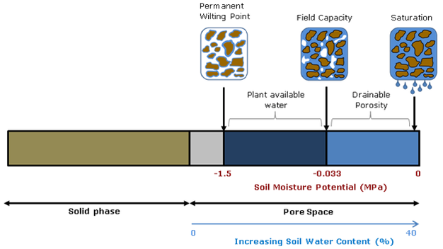
Soil moisture is critical for advancing plant and atmospheric sciences,  but the fact that different measurement techniques yield different values points to the fact that soil moisture is essentially an abstract idea.  While the water content of soil would seem to be straightforward, whether you calculate volumetric or gravimetric water content, and whether you consider chemically- and physically-immobilized water or only plant-available water (field capacity minus permanent wilting point) matters a great deal.


Diagram source.

Spatial and temporal scale also matters.  Do you want an instantaneous point measurement, or a daily weekly average for an entire county’s drought status?  Picking the right tool for the job means understanding the streghths and weaknesses of the entire gamut of technologies capable of reporting soil moisture.  This article will start with traditional in situ point measurement techniques and continue to review broad-scale soil moisture modeling and remote-sensing efforts.


from Shuttleworth 2013

Small-scale measurement can be accomplished using point-sampling with portable soil moisture probes, such as TDR and traditional (active) neutron probes.  Of course, any discussion of soil moisture measurement techniques would be incomplete without mentioning the gravimetric method, or simply weighing a soil sample wet and then dry.  But as with the other point techniques, this method can only measure hyperlocal conditions and must be replicated and averaged to inform landscape-scale management.

TDR, or time-domain reflectometry, uses the electrical properties of soil and water to calculate volumetric percent soil moisture.  For most soils, excluding those with very high organic matter (OM>10%), the TDR method without calibration provides water content in the range from zero to 50% with accuracy better than 1-2%.  While calibration and new TDR such as TRIME-TDR can improve accuracy by a factor of 10-100, the amount of microscale variability in soil means that these point measurements must be replicated dozens to hundreds of times to build up a picture of average site moisture. Microvariability can be important when precipitation preferentially flow along soil heterogeneities such as roots, textural changes, and bioturbation pathways.    Buried probes that use the TDR techniques, such as the Stevens Hydroprobes I used in my graduate research, are fixed in place and are therefore severely limited by their inability to average site variability.
  
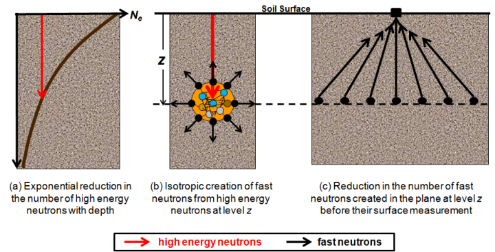
Traditional neutron probes work by bombarding the soil with high-energy neutrons and recording the number of neutrons emitted by the soil.  Hydrogen absorbs neutrons so the amount of H2O can be calculated.  This technique solves many of the problems of TDR, but the sensors are expensive and the measurement still must be repeated several times to measure field soil moisture.  

-

Meso-scale measurement can now be accomplished using the new COSMOS (Cosmic-ray Surface MOisture Sensor) program to measure whole ecosystem moisture.  Neutron moisture probes have been around for decades but COSMOS uses advances in particle-physics technology to increase sensitivity enough to rely solely on the background cosmic radiation as a uniform source of neutrons.  This advance makes possible, for the first time, instantaneous field-scale measurement of soil moisture.


These new sensors were originally deployed in 2010. They have the potential to revolutionize studies of soil moisture because they are the only technique to measure soil moisture at scales between the hyper-local point measurements and the kilometer-swaths of satellites.  They also are the only soil moisture probe that can account for water stores in living tissue.  According to Hydroinnova, one company that makes these $10,000 units, the measured soil footprint is 86% within 350 meters and the effective measuring depth changes with soil moisture, from a maximum of 70 cm in completely dry soil, to a minimum of 12 cm in saturated soil. 


Source.
While these sensors are few in number and relatively widely dispersed, they offer a whole new picture of soil moisture at the landscape level.  They are the only truly effective direct measure of soil moisture at the hectare level, and can be used to better calibrate the informational products discussed below.  However, as with all techniques, COSMOS must also be calibrated to take account of different soil types and changes in vegetation.

-

Large-scale measurement of soil moisture can be accomplished using proxies, satellites, models, or some combination of techniques.

River flow data can reveal how much water is running off or through the soil from watersheds, so using a site like the USGSstreamflow network is a good proxy for large-scale short-term drought and deluge.


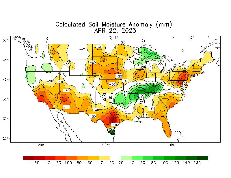
The current best methods for estimating large-scale soil moisture are the Drought.gov model products, which include the Palmer Drought Severity Index, soil moisture index, etc.  The Calculated Soil Moisture Anomaly is calculated based on observed precipitation and temperature.  Soil moisture, evaporation, and runoff for the entire US and globe are then modeled based on observations from a small area of eastern Oklahoma.  While this method is clearly biased, it is the best available.

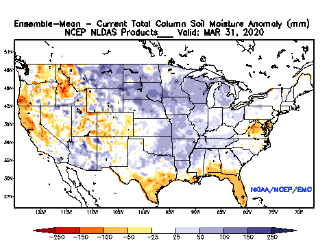
The National Land Data Acquisition System is developing a more accurate model of soil moisture that incorporates soil textural properties and average percent vegetation (which impacts evapotranspiration).  The precipitation data used in the model is at approximately 25km resolution, interpolated to 13km grid cells:


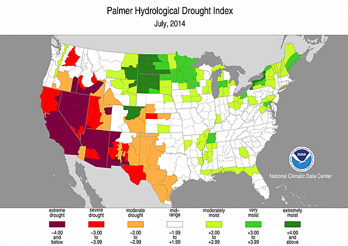
Palmer Drought Indices are similar to soil moisture models in that precipitation, evapotranspiration, and runoff are used to calculate remaining water balance.  There are long-term (Palmer Drought Index (PDI) and Palmer Hydrological Drought Index (PHDI) indices that measure changes in groundwater and reservoir levels, and short-term indices (Palmer Z Index and Crop Moisture Index (CMI)) that affect agriculture during the growing season.


 Interestingly, the US Drought Monitor, which looks essentially like one of the Palmer indices, is subjectively drawn using “a blend of science and subjectivity”.


Thursday, April 17, 2014

Water-year to Date Departure from Normal


The area East of Carlsbad, NM in Eddy county going into Lea county has had 2-4 or even 6 inches more rain than normal since October 1st.  The figure above shows that this is almost triple the normal precipitation in places. The mesquite is bright green and there are many flowers, despite below-freezing temperatures at the beginning of the week.  A good place for some springtime botany!