Why I Plan to Get the Seasonal Flu Vaccine Next Year

Introducing The Virus

Image of flu virus with antigen proteins on phospholipid(?) surface and RNA in the middle. From. http://www.cdc.gov/flu/professionals/laboratory/antigenic.htm. Tamiflu works by binding the purple neurominadse proteins. Tamiflu was developed from shikimic acid, which was originally available only as an extract of Chinese star anise but by 2006 30% of the supply was manufactured recombinantly in E. coli.[54][55]

Vaccine viruses are chosen (i.e., February for the Northern Hemisphere flu vaccine) because it takes 6-8 months to grow them in chicken eggs. Health officials would like to grow them in human(?) cell culture, but that it not currently allowed. Eggs are problematic because viruses may adapt to the egg.

"As a result, Immunologically naïve ferrets) are the most sensitive method available for detecting antigenic differences between influenza viruses."(from http://www.cdc.gov/flu/professionals/laboratory/antigenic.htm)

Evolution and Types of Virus

H3N2 (swine) flu and H1N1 (avian) flu are main lineages. Major outbreaks occur suddenly and unpredictably through transmission of new varieties from animal hosts. Seasonal (common) flus are derived from the same lineage, but generally evolve slowly and predictably. Each year, novel viruses make the leap from animal to human. For example, during the 2013–14 influenza season, one case of human infection with an new strain of H3N2v virus occurred in a child from Iowa with known direct exposure to swine. Birds seem to have co-evolved with the flu virus and do not mount an immune response to it. Therefore (luckily!) it appears to evolve much more slowly in resevoir species than in humans. This has important implications for the dynamics of seasonal and epidemic flu outbreaks.


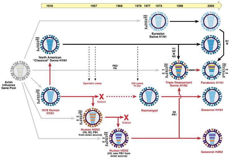
Influenza A is the most common. It is highly likely that of all the seasonal influenza strains circulating at the present, one of them will multiply and give rise to the entire seasonal influenza populations in around 5 years. The descendants of all other viruses will most likely be extinct.


For example, the 2014–15 influenza vaccines used in the United States have the same antigenic composition as those used in 2013–14. The trivalent vaccines should contain an A/California/7/2009-like (2009 H1N1) virus, an A/Texas/50/2012-like (H3N2) virus, and a B/Massachusetts/2/2012-like (B/Yamagata lineage) virus. (http://www.medscape.com/viewarticle/826572_6)

The lineage of evolutionarily successful viruses is usually termed the trunk of H3N2 influenza’s evolutionary treea:




The tree is based on hemagluttin protein sequence evolution, colored according to estimated geographic location, indicating high permanence of the trunk in China and Southeast Asia. The genetic changes occur on the neuroamidase and hemoagglutin virus surface proteins, causing antigenic drift. The truck of the H3N3 tree with a single dominant lineage contrasts with more branching trees of other flu types where different varieties often co-circulate, such as H1N1, and Influenza B and C. This graph and these findings are complicated by whole-genome sequencing: a new graph shows overall viral genome evolution in The evolution of epidemic influenza by Martha I. Nelson and Edward C. Holmes Nature Reviews.
Figure courtesy of Lemey P, Rambaut A, Bedford T, Faria N, Bielejec F, et al. http://theglobalscientist.com/2014/11/03/what-can-data-science-tell-us-about-influenza/


Current Trends - CDC FluNet


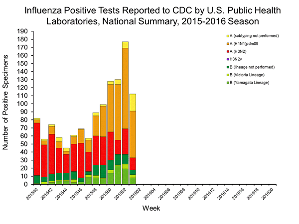
http://www.cdc.gov/flu/weekly/


Is flu increasing...

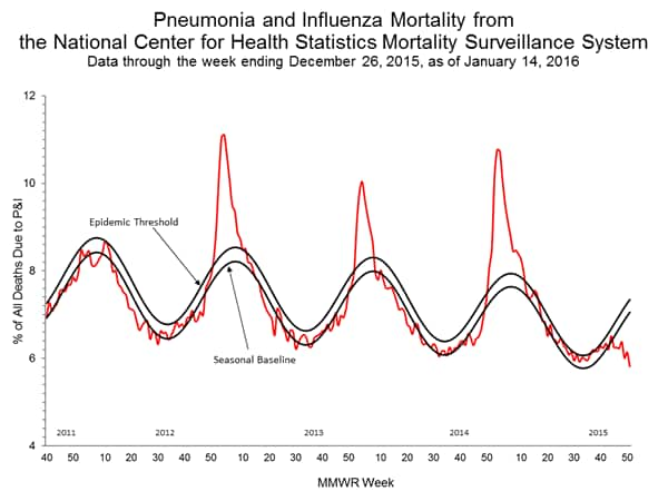
This chart is from the same page....http://www.cdc.gov/flu/weekly/. The periodicity of flu seasons and epidemics is still being studied. Peaks occur during the winter in northern latitudes at ~2–5 year intervals, usually during H3N2-dominant seasons, since the 1968 pandemic. Recent phylogenetic analysis of viruses from single populations has shown that the virus does not ‘over-summer’, but dies out at the end of each seasonal epidemic, and that subsequent seasonal viral re-emergence is ignited by imported genetic variation.

Or decreasing?

Weekly Map

http://www.cdc.gov/flu/weekly/usmap.htm

Welcome to the High Desert of New Mexico, USA

Surviving in the High Desert of New Mexico is like visiting another planet.

I suggest you find a house with a good airlock and sunshade, but you won't be able to filter out the cosmic rays; living up here is like being an airline stewardess.

The desert has a way of simplifying human needs: water, oxygen, respect (for the sun), oh, and more water.

The most important thing is water. You have to drink all the time. When you wake up in the morning you must drink a full nalgene; you've lost at least that much through exhalation during the night. I suggest miso bone broth soup to replace the electrolytes as well. Its dry here and you can't always tell when you're sweating because evaporation is so efficient.

Sometimes you can't drink enough water. The answer is coconut water. Always keep some at hand in case of emergencies.

High altitude. One of the commonest complaints (after dehydration, always check that first) is low oxygen. People forget to breathe. You have to really move that diaphragm! Ginseng and other tonifying herbs might help, too. Oh, and bone broth soup. Think like a sherpa.

Sun. I used to go without sunblock, but we're too close to the sun here. Respect the sun. Always wear sunblock when you have exposed skin - or wear a burkha. UV-blocking sunglasses are also, sadly, necessary. I hate wearing glasses, but if you don't the Light will wash away your world. Yes, it is possible to sunburn the back of your eyes.  8-(

Moisturizer. Dry skin is serious. One secret to prevent over-drying is to always end showers with cold water; it tones the muscles and closes pores in the skin so you don't lose all your hard-earned moisture. Never, ever use drying soap. I don't think that should be a problem, but I'm warning you now: Don't let cracks form on your hands or it will be Too Late, and you'll be covered in bandages like a mummy.

 Welcome to New Mexico!

Wetland, Stream, and Species Mitigation Banks

With the November 3, 2015 Presidential Memorandum "Mitigating Impacts on Natural Resources from Development and Encouraging Related Private Investment," mitigation banking has been getting more press.

Back in 2008 the US Army Corps of Engineers (USACE) and the Environmental Protection Agency (EPA) issued the 2008 Compensatory Mitigation Rule governing compensatory mitigation for activities authorized by Corps permits.  Each division of USACE has published Regional Compensatory Mitigation and Monitoring Guidelines.

Mitigation banks are restoration and conservation sites that preserve, enhance, or create important ecological functions that may be impacted elsewhere.  For example, since 2008 wetland banks can invest in the for-profit creation of new wetlands; developers can purchase credits in the bank to mitigate any impacted wetlands in the same watershed as the proposed development.

There are now over 2000 mitigation banks in the U.S.

USACE  runs the RIBITS website, which is their Regulatory in-lieu fee and bank information tracking system.

This map from RIBITS shows the distribution of mitigation banks in the continental U.S.  Some USAE districts already have dozens to hundreds of banks in operation, whereas some, such as the Albuquerque USACE district, have none.

This figure, courtesy of Kevin Janni, shows the distribution of mitigation banks and HUC watersheds in Texas for the Fort Worth and Galveston USACE districts.  Each bank may only be used to offset development within the same watershed.  Due to differing application processes and timelines for different USACE district, some districts have many more banks than others.

Mitigation banks are evaluated based on the quality of the wetlands created, using rapid assessments such as NMRAM.

The 2016 Mitigation Banking Conference will be held in Texas, May 10-13.

Ideal Amount of Potassium and Sodium Consumption to Minimize Mortality.

In the spirit of the type of analyses presented in the Perfect Health Diet, I wanted to post some correlations that appear to imply causation.  These two graphs plot Potassium and Sodium Excretion (which is assumed to be a good proxy for intake, assuming people in the study were at steady-state) versus the Odds Ratio of mortality. The odds ratio is a normalized measure of the probability of death.

The first graph illustrates that in this sample, the more potassium consumed (and hence excreted), the lower the odds ratio of mortality.

The second graph illustrates that mortality is higher for those consuming both more than, and less than, 4 g of Sodium per day.  Interestingly, the increase in mortality risk increases more slowly above 4 g/day than it does below 4 g/ day, suggesting that consuming slightly more than 4 g/ day is healthier than consuming slightly less than 4 g/day.

I think these types of analyses could be used to set standards for a whole range of vitamins, minerals, and perhaps other "Goldilocks" substances.  Goldilocks substances are things which are healthy in moderation, but either too much or too little can be harmful or hazardous.  Obviously, some substances such as toxins and radiation are inherently harmful, even down to the smallest dose (but see hormesis theory).

Source.  Urinary Sodium and Potassium Excretion, Mortality, and Cardiovascular Events N Engl J Med 2014; 371:1267 September 25, 2014.  This study looked at over 100,000 people from dozens of countries.

Bayesian Statistics

A recent post by Scientific American writer and blogger John Hogan got me thinking about Bayesian statistics again.

My favorite explanation of Bayesian statistics was by Nate Silver in The Signal and The Noise.  The basic approach involves incorporating prior estimates of probability into new measures of probability.  The opposing approach, which does not rely on prior knowledge, is termed "Frequentist" statistics and is exemplified Fisher's standard test used with p=0.05 (which implies that a given result would occur "by chance" only 5 in every 100 such tests).

Hogan uses the standard example of cancer tests to illustrate the importance and power of Bayesian thinking, but an astute commenter points out that the real power of Bayesian thinking comes when used in a process that tests, updates probabilities, and tests again, so that each test incorporates the learning from previous tests.

Silver offered a similar example in his book, but a review in the New Yorker points out that Silver got it wrong.   In Silver's case, he applies Bayesian statistics to the probability that global warming is occuring.  But the prior probability is estimated, and Bayesian approaches only improve on standard statistics when prior probabilities are well known.  So while Silver does present a rational means of updating beliefs, since the original belief is not based on statistical data, the resulting analysis cannot be called statistically valid.

Both the New Yorker review and Hogan's thoughts highlight the inherent power of confirmation bias to trump any statistical test, even Bayesian tests.

Top Conservation of Stories of 2015

Looking back on the year, I feel that victories and gained ground made good News:  US Congress acting(!) to ban microbeads,  Supreme court upheld Clean Power Plan to reduce emissions of  mercury by 1,000 million tonnes and thereby save more than 1,200 lives/year.  CO2 reduction plans from the 2015 Paris COP 16.  Administrative action to create a new office of ecosystem service financing (read: more support for restoration) and to standardize and promote mitigation banking.

However, there were some problems.  The gargantuan natural gas leak in S. Ca. highlighted the fact that natural gas leaks way too much to be a clean bridge fuel.  We either need to clean up natural gas or resolve to skip over it altogether.

A New Precipitation-Evapotranspiration Index to Map Global Drought

Standardized precipitation–evapotranspiration index (SPEI) is precipitation minus potential evapotranspiration (Vicente-Serrano et al 2010).  It is distinguished from other drought indices because it accounts for temperature through modelled evapotranspiration. This website maps global drought:

Drought in the US 2010-2011.

SPEI has recently been used to predict pine mortality in SW forests.  When the SPEI is below -1.68 for at least 11 months, pinyon and ponderosa pines cannot grow and mortality soon follows. (Kolb, T.E., 2015. A new drought tipping point for conifer mortality.Environmental Research Letters, 10(3), p.031002.)

Long-term drought graph for NM.

2015 New Mexico Weather Recap

The ABQ NWS office has an excellent recap of the state's weather over 2015.  For example, here is their summary of the summer monsoon:

The 2015 monsoon season got off to a quick start with heavy rainfall, floods, flash floods and severe weather in mid and late June, as well as the first two weeks of July.  A relatively quiet period ensued for most of the remainder of July. A resurgence of heavy rain returned from very late July through early August.  An outbreak of severe weather was the dominate weather story in mid August, and to a lesser extent on September 9th and 23rd.

By the numbers:  The Albuquerque NWS office issued 53 flash flood warnings between June 15 and September 30.

The biggest news of the year was probably the good precipitation that finally ended the drought that began in early 2011:

Drought conditions developed across New Mexico in early 2011, with few breaks in the drought through 2012, such that much of the state was gripped in the worst drought episode since the 1950s.  Near normal statewide precipitation in 2013 and 2014 did little to improve the drought.  Much of the precipitation in 2013 and 2014 fell during the monsoon season, rather than the much more needed winter mountain snowpack. Finally, New Mexico precipitation in 2015 was above normal for much of the year, and the period January through November was the fifth wettest on record since 1895.  As shown in the graph to the right, precipitation in New Mexico was well above average in January, May, July and October, with only two months below average - August and September.  These wetter than normal conditions supported a steady reduction in the intensity and coverage of the short term drought.  Finally, in early December 2015 New Mexico was drought free!  The last time the state was without any drought status was the week of November 23, 2010! By the numbers:  New Mexico went 263 weeks with a portion of the state in moderate or worse drought!
Source: U.S. Drought Monitor

A model of Ecosystem Monitoring to inform Adaptive Management

From:
Lininger, Jay.  2006. Effectiveness of Stand-Scale Forest Restoration in the Siskyou Mountains, Oregon.

NEPA Impacts Now Require Mitigation

President Obama has recently issued an important new Memorandum directing Federal agencies to employ mitigation banks to offset impacts to natural resources.

The directive re-emphasizes that agencies should seek to avoid any negative environmental impacts first, then minimize impacts, and finally, only seek compensatory offsets for harm that still occurs if necessary.  Within the limits of existing law, agencies should set ‘no net loss’ and ‘net benefit’ goals that apply to more natural resources.   (CEQ Blog Post)

The following analysis of the impacts of this memorandum are from the law office of Holland and Hart:

"We have entered a new regime in federal natural resource management, one that brings to mind Aldo Leopold’s observation that “Conservation . . . is a positive exercise of skill and insight, not merely a negative exercise of abstinence or caution.” In time, we will have a better sense of what the new regime will mean in practical terms. For now, the natural resource community will want to focus on the various agencies’ efforts to implement the directives. Across the federal government, for months to come, new rules and policies will be under development with implications for an enormous range of decisions affecting natural resources “that are important, scarce, or sensitive, or wherever doing so is consistent with agency mission and established natural resource objectives.”

These directives deserve considerable attention from those active in the natural resource law and policy arenas. There are new rules of the road for resource agency decisions subject to NEPA review, and they may significantly influence implementation of ESA and other resource protection laws. Federal resource planning efforts will likely change to include substantial consideration of “net gain/no net loss” benchmarks. Most fundamentally, the new directives seem likely to change the transactional environment facing developers seeking federal approvals for: infrastructure projects; energy, water, and mineral development; or other activities potentially impacting federal natural resources.

Agencies’ permitting and compliance decisions involve significant elements of subjectivity and uncertainty. The permitting process is often defined by bargaining over the allocation of risk between an agency wary of potentially unforeseen resource impacts and a developer or resource user wary of potentially unforeseen costs or delays. The Presidential and DOI directives can be seen as ratifying and calling for even greater effort by resource agencies to minimize or eliminate the risk of unforeseen impacts on natural resources. In effect, the agencies are being told to bargain harder, demand greater assurances, and accept little or no risk of adverse impacts when rendering decisions potentially affecting natural resources.

The directives raise the bar, but are not entirely one-sided. They encourage agencies to promote conservation banking, stewardship contracts, and other financial-incentive-based tools that generate “credits” that developers can use to offset adverse impacts of proposed projects. The internal logic of the directives appears to be that the new, higher standards for resource mitigation—net gain, or at least no net loss—are realistically achievable because any project’s unavoidable adverse impacts can be offset with conservation credits.

The agencies’ mandate to bargain harder will create difficulties for almost all resource users. To begin with, baseline resource information often lacks the empirical certainty that would make it obvious how to get to a net gain or no net loss. And what is a “net gain”? How big must that be? More challenging, the directives call for “durability” in mitigation, meaning that the quantitative and qualitative relationship of impact to compensation should endure so long as the impact continues. But natural resources change over time. Even resources that once seemed static are now recognized to be mobile as temperature, precipitation, fire, and other variables change across the landscape. The new directives will particularly frustrate those resource users who are not inclined to anticipate nor internalize within their project planning and business judgments the agencies’ resource management goals. Whatever the agencies were bargaining for yesterday, they’ll soon be bargaining for more.

There is something encouraging here for those resource users who approach the regulatory environment with a transactional mindset. The directives’ embrace of compensatory mitigation means that, once the directives have had time to be incorporated into agency procedures, there should be a predictable regulatory “solution” for a project potentially posing the risk of adverse resource impacts. In theory, the ultimate decision about whether - and on what terms - to approve a permit or other authorization should be somewhat less vulnerable to an agency official’s reluctance to countenance unavoidable adverse resource impacts. This is particularly so if the agencies do, in fact, embrace the use of mitigation banks and other credit-generating tools.

The other potential winners from the directives will be private investors in mitigation banks and similar financial structures that produce resource “credits” to exchange for impacts.