Wildlife Trends in Arizona: 150 Years of Winner and Losers

 Arizona’s wildlife history is an example of a timeline that occurred in many developing landscapes: an era of exploitation and eradication (1800s–1950s) followed by an era of restoration and management (1980s–present). 

However, there are some factors that were unique to the United States that led to distinct trends in wildlife populations when compared to those same species across the border in Mexico.

The following summary of research (Part 1) lists 16 Arizona species that were extirpated or greatly reduced and whether they have recovered.  Part 2 looks at 10 species that occur in both Arizona and Mexico and why their populations followed different trends.

This research illuminates the current state of wildlife and ecosystems in Arizona and helps explain the factors that got us here.

Part 1: Arizona vs. Wildlife

The following summary organizes species into groups based on their population trajectories: the “Great Returns” that were extirpated but have been successfully reintroduced, the “Survivors” that have been greatly reduced but still persist, and the “Lost Causes” that were extirpated but have not been successfully reintroduced. 

I. The "Great Returns": Extirpated & Successfully Reintroduced

These species were completely removed from the state but have been restored, often using proxy subspecies or captive breeding.

Rocky Mtn Elk

Extirpation Date/Cause: 1900: The native Merriam’s subspecies was hunted to extinction for meat and teeth.

Reintroduction Date/Area: 1913–1928: Rocky Mtn elk from Yellowstone were released near Winslow, Alpine, & Kingman.

Key Trend/Notes: Ecological Substitution: A proxy subspecies filled the empty niche, expanding rapidly due to lack of competition.

Mexican Gray Wolf

Extirpation Date/Cause: 1970: Eradicated by federal predator control programs (poison/traps) to protect livestock.

Reintroduction Date/Area: 1998: Captive-bred wolves released in the Blue Range Primitive Area.

Key Trend/Notes: Predator Tolerance: Success is biologically high but socially controversial; relies on ongoing conflict management.

 

California Condor

Extirpation Date/Cause: 1924: Vanished due to lead poisoning (bullets in carrion) and shooting.

Reintroduction Date/Area: 1996: Released at Vermilion Cliffs.

Key Trend/Notes: Intensive Care: Survival relies on active management (chelation therapy for lead) rather than self-sufficiency.

River Otter

Extirpation Date/Cause: 1950s: The native Sonora subspecies was  trapped out for fur.

Reintroduction Date/Area: 1981–1983:  Louisiana subspecies released in the Verde River.

Key Trend/Notes: Another Proxy: Like the elk, a non-native subspecies was used to successfully fill the vacant ecological role.

Black-footed Ferret

Extirpation Date/Cause: 1960s: Poisoning of their food source (prairie dogs) led to total extirpation.

Reintroduction Date/Area: 1996: Reintroduced in Aubrey Valley (Seligman).

Key Trend/Notes: Disease Barrier: Success is limited by sylvatic plague; requires dusting burrows and vaccines to persist.

Apache Trout

Extirpation Date/Cause: Mid-1900s: Hybridization with non-native rainbow trout and habitat loss.

Reintroduction Date/Area: 1955–Present: White Mtns (managed by White Mountain Apache Tribe & AZGFD).

Key Trend/Notes: The First Win: Became the first sportfish in history to be delisted from the Endangered Species Act (2024).

 

II. The "Survivors": Reduced but Persisted

These species were decimated by unregulated market hunting or predator control but survived in rugged refugia (escape terrain).

Desert Bighorn

Historic Low Point: Early 1900s: Reduced by diseases from domestic sheep and market hunting.

Survival Factor: Terrain: Survived in the most inaccessible desert peaks (Grand Canyon, Kofa).

Current Status: Translocated: Populations are moved to historic ranges (e.g., Santa Catalinas, Virgin River) to ensure genetic diversity.

 

Mountain Lion

Historic Low Point: 1960s: Bountied as "vermin" until 1970.

Survival Factor: Elusiveness: Solitary nature and rough terrain made total eradication impossible.

Current Status: Stable: Managed as a big game species; populations are robust statewide.

Beaver

Historic Low Point: 1890s: Trapped out of major rivers (San Pedro, Santa Cruz).

Survival Factor: Cryptic Behavior: Survived in deep canyons (Verde/Black River) by using bank burrows instead of lodges.

Current Status: Recovering: Reintroduced to the San Pedro (1999); used today for watershed restoration.

Pronghorn

Historic Low Point: 1920s: Fences cut off migration; market hunting reduced herds.

Survival Factor: Open Space: Remnant herds survived in vast private ranchlands (Babbitt Ranches).

Current Status: Managed: Sensitive to habitat fragmentation; relies on modifying fences for movement.

Gunnison’s Prairie Dog

Historic Low Point: 1930s: Poisoned across vast areas.

Survival Factor: Remote Refugia: Survived in the high-elevation Aubrey Valley; resistant to plague.

Current Status: Keystone: Their persistence allowed the Black-footed Ferret reintroduction to happen.

 

III. The "Lost Causes": Extirpated & Failed (or Struggling) Reintroductions

Complex social behaviors or specific habitat needs made simple reintroduction impossible.

Thick-billed Parrot

Extirpation Cause: 1938: Shooting/Poaching.

Reintroduction Outcome: Failed (1986–93): Chiricahua Mtns.

Why It Failed: Cultural Knowledge: Captive birds lacked flock wisdom to avoid hawks and find food.

Masked Bobwhite Quail

Extirpation Cause: 1900: Cattle overgrazing destroyed tallgrass cover.

Reintroduction Outcome: Struggling (1937–Present): Buenos Aires NWR.

Why It Failed: Habitat Specificity: Reintroduced birds often die due to lack of specific cover and predation; almost entirely reliant on captive releases.

Gila Topminnow

Extirpation Cause: 1940s: Invasive Mosquitofish.

Reintroduction Outcome: Mixed/Struggling: Multiple failures in the 80s/90s.

Why It Failed: Invasive Barrier: Cannot survive where aggressive non-native fish are present.

Jaguar

Extirpation Cause: 1963: Killed as predator.

Reintroduction Outcome: Natural Transients Only: No formal reintroduction.

Why It Failed: Political/Social: Only solitary males currently cross from Mexico; no breeding population exists.

Grizzly Bear

Extirpation Cause: 1936: Killed as predator.

Reintroduction Outcome: Permanently Extirpated.

Why It Failed: Social Tolerance: Requires vast, roadless wilderness that no longer exists in AZ; no plans to reintroduce.

 

Unifying Trends in Arizona Wildlife History:

The Predator Paradox:

Predators (wolves, grizzly bears and black bears, jaguars, lions) were targeted by federal policy for eradication to protect livestock.  Only the cryptic/solitary ones (lions, bears in rough terrain) survived. Reintroducing social predators (wolves) has been biologically successful but socially difficult.

The Proxy Solution:

When a native subspecies was completely lost (Merriam's Elk, Sonora Otter), biologists successfully substituted a close relative (Rocky Mtn Elk, Louisiana Otter).  These ecological substitutes often thrived because the niche was wide open and they were generalists.

The Behavioral Barrier:

Reintroductions of intelligent, social animals (Thick-billed Parrot) or habitat specialists (Masked Bobwhite) often fail.  Hard releases (letting animals go) work for generalists like elk but fail for species that require learned behavior or specific micro-habitats.

Part 2: Arizona vs. Mexico

This analysis breaks down Arizona’s extirpated and reduced species by comparing them to their source populations in other U.S. states and their often-distinct fates across the border in Mexico.

The overarching trend reveals a paradox: while the U.S. effectively managed game species (elk, sheep) through public land regulation, Mexico’s private land system (ranchos) inadvertently served as the final lifeboat for nongame species (wolves, prairie dogs, parrots) that were systematically eradicated in the U.S.

Successful Reintroductions: The Game Bias

The species that succeeded in Arizona were often abundant elsewhere in the U.S. but had been wiped out or severely reduced in Mexico.

Rocky Mtn. Elk

Status in Other U.S. States: Thriving: Millions exist across the Rockies (CO, MT, ID).

Status in Mexico: Extirpated / Rare: Native Merriam’s were also lost in Mexico. Small, private herds of Rocky Mtn. elk exist now on high-fence ranches in Coahuila/Sonora.

Accounting for the Difference: Public Land Management: The U.S. model of public land hunting funded the massive translocation efforts. Mexico lacked the public land base or agency funding to replicate this scale of reintroduction.

River Otter

Status in Other U.S. States: Secure: Abundant in the Mississippi Delta and Pacific Northwest.

Status in Mexico: Critical / Extirpated: The native Sonora otter is likely extinct in the Colorado River Delta due to the complete drying of the river before it reaches the sea.

Accounting for the Difference: Water Policy: Arizona’s otters survive in protected flows (Verde/Salt). In Mexico, the water is siphoned off for agriculture before it can support otter habitat.

Mexican Gray Wolf

Status in Other U.S. States: Extirpated: Historically ranged into NM/TX (now reintroduced there).

Status in Mexico: Reintroduced (Struggling): Mexico began releasing wolves in the Sierra Madre in 2011. The population is smaller and more fragile than the AZ/NM population.

Accounting for the Difference: Prey Base: In Arizona, wolves rely on abundant elk. In Mexico, elk are absent and deer are scarcer, forcing wolves to target livestock, leading to immediate conflict with ranchers.

Reduced/Survivors: The Refugia Divide

Species that held on in Arizona often did so in rugged terrain, while in Mexico, their fate depended heavily on the stewardship of individual landowners.

Desert Bighorn

Status in Other U.S. States: Stable: NV, CA, and UT have strong, managed herds.

Status in Mexico: Stable / Commercialized: In Sonora and Baja, bighorn are a high-value commodity. Private ranchers protect them aggressively to sell high dollar hunting tags ($50k+).

Accounting for the Difference: Economic Incentive: In the U.S., bighorn are protected by state agencies as a public trust. In Mexico, they survived because they became a private asset worth protecting from poachers.

Pronghorn

Status in Other U.S. States: Secure: WY and MT have massive herds.

Status in Mexico: Endangered (Sonoran Subspecies): The Sonoran Pronghorn (El Pinacate) is critically endangered.

Accounting for the Difference: Barriers: The U.S. herds had open range. The Mexican herds were hemmed in by highways (Hwy 2) and border fencing, severing their ability to find water during droughts.

Beaver

Status in Other U.S. States: Abundant:  r egained range across the West.

Status in Mexico: Recovering (Delta): The Colorado River Delta saw a miraculous, short-term return of beavers following the "Pulse Flow" (Minute 319) water release in 2014.

Accounting for the Difference: Resilience: Beavers in Mexico proved they are waiting in the wings; they only lack the water, whereas U.S. populations had consistent flows in mountain refugia.

Failed/Struggling: The Mexican Lifeboat

Species that failed in Arizona (often due to poisoning or habitat loss) survived in Mexico, which served as the last stronghold.

Masked Bobwhite

Status in Other U.S. States: Extirpated: Only exists in captivity/refuge.

Status in Mexico: Critical / Persistent: Small wild populations were rediscovered on private ranches in Sonora (e.g., Rancho Carrizo) in the late 20th century.

Accounting for the Difference: Grazing Intensity: While U.S. ranchers switched to exotic grasses (Lovegrass), some remote Sonoran ranches maintained native vegetation due to isolation and traditional (lower intensity) grazing practices.

Thick-billed Parrot

Status in Other U.S. States: Extirpated: No wild flocks in the U.S.

Status in Mexico: Endangered / Extant: ~2,000 birds breed in the Sierra Madre Occidental (Chihuahua/Durango).

Accounting for the Difference: Old Growth Timber: Arizona logged its sky island nesting snags by the 1930s. The remote Sierra Madre retained old-growth forests longer (though these are now threatened by logging).

Jaguar

Status in Other U.S. States: Extirpated: (Breeding populations).

Status in Mexico: Vulnerable / Breeding: A reproducing population exists in Sonora (Northern Jaguar Reserve), only ~120 miles south of the border.

Accounting for the Difference: Road Density: Arizona is crisscrossed by paved roads and development. The Sonoran habitat is more rugged, roadless, and largely privately owned, reducing human-cat interaction.

Black-tailed Prairie Dog

Status in Other U.S. States: Extirpated: Widespread poisoning campaigns.

Status in Mexico: Thriving (Janos): The Janos Biosphere Reserve in Chihuahua holds one of the largest prairie dog complexes in North America.

Accounting for the Difference: Benign Neglect: The U.S. government funded industrial-scale poisoning. The Mexican government lacked the funds for such programs, inadvertently allowing the massive colonies to survive until conservationists bought the land.

Summary of Differences

The Industrial Efficiency of Extirpation

Arizona’s extirpations were often more thorough than Mexico’s because the U.S. had the resources to be efficient. Government-sponsored predator control (wolves/jaguars) and poisoning (prairie dogs) were well-funded industrial operations in Arizona. Mexico, lacking these centralized resources, allowed "pest" species to survive simply through "benign neglect."

Public vs. Private Conservation

Arizona: Success relies on public land management (US Forest Service/BLM). This is great for generalists like elk but hard for specialists that need specific micro-habitats.

Mexico: Survival has relied on private land isolation. Remote ranches in the Sierra Madre acted as unintended nature preserves because they were too difficult to log or develop.

The Elk Gap

The single biggest ecological difference today is elk. Arizona replaced its lost native elk with a massive, successful herd of Rocky Mountain elk. Mexico never did. This means Arizona has a massive prey base for wolves and lions that Mexico lacks, creating a "food imbalance" at the border that complicates predator recovery in the south.

 

DNA Barcodes, Klee Diagrams, and the Secrets of Speciation

Modern biodiversity detectives have found new ways to synthesize massive amounts of sequence data into clear information and insights. Two powerful tools to help visualize and understand the structure of life are DNA barcodes and Klee diagrams. Mark Stoeckle and David Thaler pioneered the use and explanation of these tools to offer insights into how species originated and evolved.

What is a DNA Barcode?

A DNA barcode is a short, standardized segment of the genome used for species identification. In the animal kingdom, the gold standard is a 648-base pair (bp) segment of the mitochondrial cytochrome c oxidase subunit I (COI) gene. While this segment represents less than one-millionth of an organism’s total genome, it has proven remarkably effective because mitochondrial DNA clusters largely overlap with species as defined by experts.

This tool is commonly used in eDNA samples to identify species from the environment. The BOLD (Barcode Of Life Database) now contains approximately five million of these barcodes, covering about 100,000 animal species. Interestingly, there is nothing inherently “special” about the COI gene biologically; it became the standard because reliable primers were adopted by a critical mass of the scientific community.

Visualizing Life: The Klee Diagram

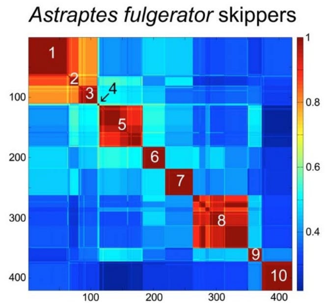
To make sense of these millions of sequences, scientists developed the Klee diagram, a heat map that displays correlations between DNA sequences. In these diagrams, every sequence is compared with every other sequence, and the intersections are color-coded to show similarity. (Sirovich, Lawrence, Mark Y. Stoeckle, and Yu Zhang. “Structural analysis of biodiversity.” PLoS One 5.2 (2010))

Species-level clusters in skipper butterfly Astraptes fulgerator COI barcode Klee diagram. Sequence clusters appear as blocks of high correlation along the diagonal and correspond to the 10 provisional species (1. INGCUP, 2. HIHAMP, 3. FABOV, 4. BYTTNER, 5. YESENN, 6. LONCHO, 7. LOHAMP, 8. SENNOV, 9. CELT, 10. TRIGO). Block sizes reflect number of sequences per species (n 3–88). Stoeckle and Coffran 2013.

Key features of Klee diagrams include:

• Indicator Vectors: Each DNA sample is listed on both the x and y axis and a heat map is generated comparing each species to itself (red=1, a perfect match) and all of the other samples in the database.

• Species Islands: When sequences are arrayed, species appear as sharp, non-overlapping squares. This visualization confirms that species are “islands in sequence space,” with distinct clusters and empty gaps between them.

• Scalability: Recent software developments like PyKleeBarcode allow these diagrams to be computed for very large datasets, potentially representing the whole animal kingdom in a single information space.

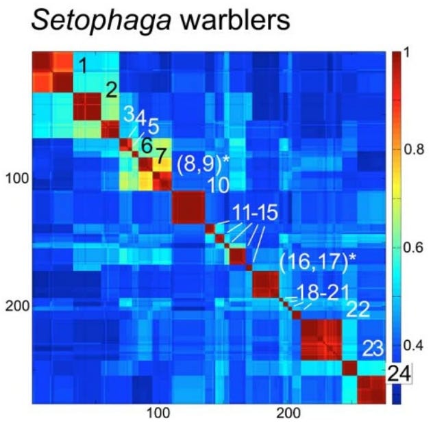
Species-level clusters in birds: Setophaga warblers COI barcode Klee. Blocks along the diagonal correspond to species; species with shared blocks are marked with an asterisk (1. petechiae, 2. striata, 3. pensylvanica, 4. nigrescens, 5. graciae, 6. discolor, 7. virens, 8. occidentalis,* 9. townsendi,* 10. magnolia, 11. tigrina, 12. castanea, 13. dominica, 14. palmarum, 15. citrina, 16. americana,* 17. pitiayumi,* 18. cerulea, 19. pinus, 20. kirtlandii, 21. fusca, 22. coronata, 23. caerulescens, 24. ruticilla). Stoeckle and Coffran 2013.

Evolutionary Implications: Why Mitochondria Define Species

A long controversy in biology concerns whether species are “real” or just human constructs. Dobzhansky, in his 1937 book Genetics and the Origin of Species, claimed that “Biological classification [of species] is simultaneously a man-made system of pigeonholes devised for the pragmatic purpose of recording observations… and an acknowledgement of the fact of organic discontinuity.”

Stoeckle and Thaler, in their 2018 paper “Why should mitochondria define species?”, expand on the evolutionary meaning behind these barcode clusters. They argue that the patterns seen in DNA barcodes are central facts of animal life that evolutionary theory must explain.

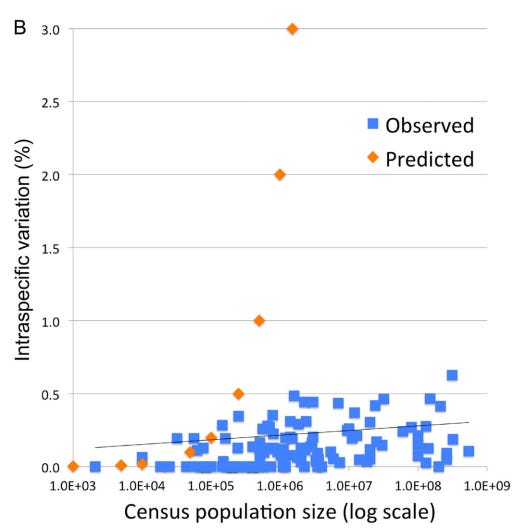
1. The “Barcode Gap” and Low Intraspecific Variation: Across the animal kingdom, the average pairwise difference (APD) within species is typically very low, between 0.0% and 0.5%. Meanwhile, the distance between even the most closely related species is usually 2% or more. This “gap” exists because intermediates between clusters are absent or rare.

2. The Neutrality of Synonymous Mutations: Most variation within and between these barcode clusters consists of synonymous substitutions; mutations that change the DNA sequence but not the resulting protein.

Stoeckle and Thaler argue that these changes are selectively neutral in mitochondria. This is because animal mitochondria are simpler than the nuclear genome; they lack introns (and thus splicing) and only have 22 different tRNA types. This lack of complexity means synonymous codons are less likely to affect the “fitness” of the organism, allowing them to accumulate as a “molecular clock”.

However, observed patterns of variation in DNA barcodes do not match the predictions of Kimura’s Neutral evolutionary theory of random accumulation of mutations.

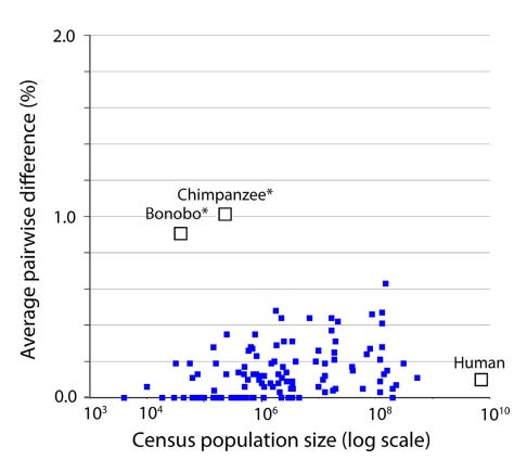
Intraspecific variation and population size among 111 bird species with census estimates; species with geographic or hybrid clusters were excluded. Orange markers indicate predicted variation for a model species under neutral evolutionary drift. Stoeckle and Thaler 2014.

3. A Recent Universal Expansion? To reconcile these observations, Stoeckle and Thaler’s use humans as a case example. Modern humans have an APD of 0.1%, which is about average for the animal kingdom.

Several lines of evidence suggest that human mitochondria originated from a state of uniformity approximately 100,000 to 200,000 years ago before expanding. Stoeckle and Thaler propose that the extant populations of humans, and almost all other animal species, arrived at a similar result due to a similar process of expansion from mitochondrial uniformity within the same recent geological timeframe.

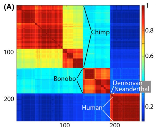
Klee diagram of mitochondrial genetic diversity of humans and our closest living and extinct relatives. The human sequences represent the span of known modern diversity. The Klee diagram heat map demonstrates greater mitochondrial diversity among chimpanzees and bonobos than among living humans. Thaler and Stoeckle 2016.

This coincides with Mayr’s 1942 idea that bottlenecks followed by expansion could explain speciation:

“The reduced variability of small populations is not always due to accidental gene loss, but sometimes to the fact that the entire population was started by a single pair or by a single fertilized female. These “founders” of the population carried with them only a very small proportion of the variability of the parent population. This “founder” principle sometimes explains even the uniformity of rather large populations…”

Mitochondrial genetic diversity, represented as average pairwise difference of COI barcodes, in relation to census population size in humans, chimpanzees, and bonobos compared to a well characterized set of birds (Stoeckle and Thaler 2014). Mitochondrial genetic diversity in humans is about 0.1%, less than that of many bird species, despite having more than 10-fold greater population than the most abundant bird in this dataset. Chimpanzees and bonobos have much smaller population sizes than humans, but conspicuously higher diversity, consistent with reproductively isolated subgroups. Thaler and Stoeckle 2016.

Conclusion

DNA barcodes and Klee diagrams do more than just identify species; they reveal a kingdom-wide pattern of organic discontinuity. Whether through population bottlenecks, lineage sorting, or gene sweeps, the uniform low variance across species suggests that the “islands” of biodiversity we see today are the result of deep evolutionary currents that affect all animals—from humans to birds to insects—in a surprisingly similar way.

Thaler and Stoeckler conclude their 2018 paper by noting that “there is irony but also grandeur in this view that, precisely because they have no phenotype, synonymous codon variations in mitochondria reveal the structure of species and the mechanism of speciation.”

Annotated Bibliography

Sirovich, Lawrence, Mark Y. Stoeckle, and Yu Zhang. “Structural analysis of biodiversity.” PLoS One 5.2 (2010): e9266.

- lays out math and originally defines “Klee diagrams”. Some examples.

Stoeckle, Mark Y., and Cameron Coffran. “TreeParser-aided Klee diagrams display taxonomic clusters in DNA barcode and nuclear gene datasets.” Scientific Reports 3.1 (2013): 2635.

- short and sweet version for Nature. Butterly and Warbler Klee examples.

Stoeckle, Mark Y., and David S. Thaler. “DNA barcoding works in practice but not in (neutral) theory.” PLoS one 9.7 (2014): e100755.

- first paper to note that the observed patterns in Klee diagrams, of homogenous species, doesn’t match neutral theory. OK.

Thaler, David S., and Mark Y. Stoeckle. “Bridging two scholarly islands enriches both: COI DNA barcodes for species identification versus human mitochondrial variation for the study of migrations and pathologies.” Ecology and Evolution 6.19 (2016): 6824-6835.

- short but good paper, cool data on humans, bonobos, and chimps, and comparison to results from their 2014 paper disproving neutral theory. Human/Chimp Klee example.

Stoeckle, Mark Y., and David S. Thaler. “Why should mitochondria define species?.” BioRxiv (2018): 276717.

- deep dive analysis that builds on 2014 observation that mitochondrial DNA barcodes don’t match expectations of neutral theory (”Species are islands in sequence space.”), while at the same time appearing to be created by neutral (synonymous) sequence changes. This is explained by evolutionary mechanisms of speciation, which has implications for how recent most species have become species. These results also help to resolve some of the disagreements about the definition of a species.

Duchemin W, Thaler DS (2023) PyKleeBarcode: Enabling representation of the whole animal kingdom in information space. PLOS ONE 18(6): e0286314.

- methods paper

Porcupines in Arizona

An Arizona Porcupine observed at Willow Lake in Prescott.  Link to iNat observation.  

Porcupines are infrequently observed in Arizona, with only 206 total observations on iNaturalist since 2009, of which 198 are positively identifiable.  (Compared to about 900 observations in New Mexico.)  

Of the 198 in Arizona, 35 were at Willow Lake in Prescott, 55 at Petrified Forest National Park in NE Arizona, and about 30 between Williams and Flagstaff.  The remaining 78 were observed in ecosystems across the state, except for the Sonoran desert.

102 were observed on the ground, but 24 were dead, and half of those (6% of the total) were roadkill (viewer discretion advised).

Porcupine dead on road in Prescott.  Link to iNat observation.

96 porcupines were observed using different tree species as habitat.  The most common tree was cottonwood (Populus fremontii), followed by Ponderosa Pine (Pinus brachyptera).  Willows (Salix goodinggii) were also frequent.  Porcupines were observed in all common tree species, including oaks (Quercus), Junipers (Juniperus), Pinyon pines, Elms, and Douglas Fir (Pseudotsuga menziesii).  

Porcupine in cottonwood tree, Willow lake. Link to iNat observation. 

Acid-Base Balance: Foods and Supplements

I previously wrote about the role lactic acid can play in disease.  This raised the question of whether foods and supplements can buffer metabolic acidity.  If so, which foods or supplements are most beneficial?  Does pH correlate to the effect on the acid-base balance of the body?

This is important because:

• Chronic acid load can deplete alkalinizing minerals, leading to e.g. calcium bone loss.
• Long Covid may be caused by metabolic acidosis: https://researchaidnetworks.org/hypothesis-summary/

After researching this, I concluded that a food's pH does not directly correlate with its impact on overall acid base balance.  Potential Renal Acid Load (PRAL) is determined by mineral and protein composition, not its inherent acidity.  

For example:

• Lemons taste acidic due to citric acid, but have a negative PRAL (alkaline-forming) because they're rich in potassium and other compounds that generate bicarbonate when metabolized
• Animal proteins may not taste acidic but have a high positive PRAL (acid-forming) due to sulfur-containing amino acids that get metabolized to sulfuric acid.

The key biochemical factors that determine a food's PRAL include:

1. Protein content (especially sulfur amino acids) - metabolized to produce acids
2. Mineral content: 
1. Potassium, calcium, magnesium - metabolized to produce bicarbonate (alkaline)
2. Phosphorus, chloride - contribute to acid load
3. Organic acid content - intermediates in the citric acid cycle (Krebs cycle), their oxidation generates bicarbonate. Each molecule of malate or citrate metabolized can generate multiple bicarbonate molecules.

Details

The pH of urine is influenced by the body's metabolic acid load and the kidney's ability to regulate hydrogen ion (H⁺) excretion.  The kidneys play a crucial role in maintaining acid-base balance by adjusting the amount of hydrogen ions eliminated or retained.  When the body experiences a metabolic acid load, the kidneys respond by increasing H⁺ excretion. This lowers urine pH, reflecting the increased acid load on the body.  However, positive cations can also stimulate renal acid-base regulation, leading to increased hydrogen ion excretion (and bicarbonate (HCO₃⁻) regeneration).  This results in a decrease in urine pH, even as the body experiences a reduced metabolic acid load.

Cations can also activate enzymes that convert metabolic acids to bicarbonate.  The more positively charged the cation, the more efficiently it can displace hydrogen ions.

Organic acid conjugation to cations enhances alkalinization.  For example, citrate enters the citric acid cycle directly and generates multiple bicarbonate (HCO₃⁻) upon oxidation.

Table of Common Supplements and Food Additives; their pH and effect on acid-base balance.  

This data shows how solution pH and PRAL effects don't always correlate. For example, while KCl has a neutral pH in solution, it has a slightly negative PRAL due to the potassium content. However, extreme pH (either acid or base) can correlate with PRAL effect.

Categories of Supplements

1. Neutral pH, Alkalizing Effect: 
1. Potassium citrate
2. Calcium lactate
3. Potassium gluconate
4. These demonstrate the pH vs. physiological effect paradox
2. Mineral-Organic Complexes: 
1. Magnesium citrate and malate show slightly acidic pH but strong alkalizing effects
2. Zinc citrate has less alkalizing effect despite similar pH
3. Simple Salts: 
1. KCl shows neutral pH with mild alkalizing effect
2. NaCl shows neutral pH and neutral physiological effect
4. Strong Acids/Bases: 
1. HCl, KOH, NaOH show correlation between pH and physiological effect
2. These are exceptions to the general trend of pH not predicting physiological impact

Alkalinizing Potential Ranking

The formula for PRAL (mEq/100g) is: PRAL = 0.49 × protein (g) + 0.037 × phosphorus (mg) - 0.021 × potassium (mg) - 0.026 × magnesium (mg) - 0.013 × calcium (mg).  

Negative PRAL indicates an alkalizing effect on the body.

Example:  mice

Mice diets were compared using Dietary Cation Anion Balance (DCAB), a similar metric to PRAL.  DCAB is calculated by adding the weighted amount of acidifying anions and alkalizing cations in the diet. 

It has been shown in many species that the dietary cation anion balance (DCAB) influences acid base homeostasis and urine pH.  With the DCAB, the resulting urinary pH can be predicted with species-specific equations. 

DCAB [mmol/kg DM] = 49.9 · Ca + 82.3 · Mg + 43.5 · Na + 25.6 · K − 59.0 · P − 62.4 · S − 28.2 · Cl; mineral content in g/kg DM.  (Negative DCAB indicates an acidifying effect on the body.)

The paper found that a negative DCAB results in metabolic acidosis, and "Fed long-term, this can contribute to the reduction of bone mineral density due to a PTH-mediated increase in renal calcium excretion. Metabolic acidosis also induces renal phosphorus excretion, resulting in hypophosphatemia."

Citation: https://www.mdpi.com/2076-2615/11/3/702 

Böswald, L.F.; Matzek, D.; Kienzle, E.; Popper, B. Influence of Strain and Diet on Urinary pH in Laboratory Mice. Animals 2021, 11, 702. https://doi.org/10.3390/ani11030702

Example:  human athletes

Alkaline water has demonstrated its effectiveness as an alkalizing agent in the treatment of metabolic acidosis in both animal and human research. Past studies have shown that daily intake of 2.5–4 L of alkaline water for 3~6 weeks has significant impacts on anaerobic performance and acid–base balance in athletes.  This study showed that alkaline water co-ingested with glutamine led to decreased stress markers in athletes.  Masterjohn hypothesizes that glutamine is converted to glutamate to buffer lactic acid in muscles, and that decreasing PRAL contributes to more available glutamine for other metabolic functions..  

Citation: https://www.mdpi.com/2072-6643/16/3/454

Lu, T.-L.; He, C.-S.; Suzuki, K.; Lu, C.-C.; Wang, C.-Y.; Fang, S.-H. Concurrent Ingestion of Alkaline Water and L-Glutamine Enhanced Salivary α-Amylase Activity and Testosterone Concentration in Boxing Athletes. Nutrients 2024, 16, 454. https://doi.org/10.3390/nu16030454

Thanks to Claude Sonnet for back-and-forth conversation, and for creating the table and figure above.  

Are Pollinators Necessary for Food Production?

Pollinator enthusiasts claim that "1 in 3 bites of food are dependent on pollinators", but the reality is that many crops have been bred to self-pollinate.  For example, soybeans produce bean-like flowers, and many wild beans do require insect pollinators, but soybean flowers never open; they self-pollinate.  

In the wild, 70-90% of flowering plant species (angiosperms) do require an animal (usually an insect, bird, or mammal) to move pollen from one flower to another. Source. Only a few species have evolved to become self-reliant or to rely on wind.  But in human agriculture, we've selected for species that "breed true", which often means selecting for self-pollination. 

Many flowering agricultural crops would appear to need pollinators, but don't.  Or at most the pollination is optional: it doesn't hurt for insects to visit the flowers, and sometimes they help to fertilize and hence set more fruit, but they aren't strictly needed.  Although about three-quarters of crops benefit in some way from animal pollination, only about 10 % depend fully on pollinators to produce the seeds or fruits we consume, and they collectively account for only 2 % of global agricultural production. Source.

I created this table to show the AZ crops that require pollinators.

Data from Our World in Data: https://ourworldindata.org/pollinator-dependence

More information: https://en.wikipedia.org/wiki/List_of_crop_plants_pollinated_by_bees

The Problem with Nutrigenomics

"Personalized nutritional counseling is a burgeoning field. Several companies, including Vitagene, Nutrigenomix and DNAFit, are already offering individualized dietary counseling.  Their efforts are based mostly on genetic testing, but scientists have only just begun to explore the links between DNA and good nutrition. “I think companies offering personalized dietary advice are probably running ahead of the evidence,” said John Mathers, director of the Human Nutrition Research Center at Newcastle University in Britain." [NYTimes Blog]

Introduction

Science skeptics have recently reviewed these services, and found plenty of quackery. [Science Based Medicine] [Skeptical Raptor]

However, there is some research to back up the idea that genetic testing can provide insights into metabolic disorders.  There may be as many as 200 SNPs for which there are proven metabolic effects, and only a subset of these alter nutrient requirements in a significant portion of the population [e.g., the rs1801133 MTHFR SNP and folate requirement in 15–30% of the population (Solis et al., 2008) and the rs12325817 PEMT SNP and choline requirement in 20–45% of the population (da Costa et al., 2006)].

What do genetic testing services measure?

The human genome consists of about 3 billion nuceleotide bases, each of which is either A,C, T, or G.  A reference genome based on the similarities of all genotyped humans has been assembled, along with a corresponding reference database of all of the point "mutations" where individuals differ from that baseline.  So far, scientists have documented about 150 million of these single nucleotide polymorphisms, called SNPs.  The average person doesn't have all of these differences, however; most people have about 3 millions SNPs that differentiate them from the reference human genome.   Since 3 million is about 0.1% of the 3 billion base pairs, most humans differ from each other by about 0.1% of our DNA. Ancestry genomic testing services like 23andme test for a few hundred thousand SNPs for $100-$200.  For $1000-10,000 a complete genomic sequence can be obtained.  (there are about 3 billion bases total.  

Examples: MTHFR – metabolic pathways and nutrigenomics

In humans, SNPs in the gene MTHFD1 increase the demand for betaine as a methyl-donor, thereby increasing the dietary requirement for choline. Another SNP in the gene PEMT prevents the activation of this gene by estrogen, thereby decreasing endogenous production of phosphatidylcholine (a source of choline) in the liver and increasing the dietary requirement for choline. [Choline: Critical Role During Fetal Development and Dietary Requirements in Adults. Ziesel]

But note that it is not so simple.  There are several forms of the MTHFD1 gene, for example MTHFD1L and MTHFD2. If MTHFD1 is commonly mutated, it may be a pseudogene.

Complexities interpreting SNPs

No simple test can unravel the intricacies of the human genome, and consumers should be suspicious of anyone claiming to be able to interpret measurements of tens of thousands of genes, with millions of genetic variations, some of which have effects on hundreds or thousands of the small molecules of metabolism (and perhaps on thousands of peptides or proteins involved in metabolism).

[A grand challenge for nutrigenomics.  Steven Zeisel. 2010.]

Mistakes in genomics data

Note that 23andme data, like any large genome scan, can have mistakes in it.  For example, the Enlis genomics blog found more than 500 likely mistakes in a sample of 23andme raw data!  (Enlis)

Furthermore, many important nutritional SNPs are not testing by 23andme.

Solution: Metabolic Testing
There is a genetic test for MTHFR variations. But there’s also a cheaper and more accurate way to test for whetherMTHFR variations are causing disease. We simply check the levels of homocysteine in the blood...In other words, the homocysteine levels determine our actions, not the MTHFR test results.[Cleveland Clinic]

Testing a Relevant SNP?

A new study in Science Magazine by Simonti et al has linked this SNP to a rare condition known as protein-calorie malnutrition (PCM).  The study compared electronic health records (EHR) for 28,000 people with SNPs that are now known to derive from Neandertal DNA.

SNP rs12049593 is in an intron of SLC35F3, which means it does not change the actual structure of the protein, but instead alters the amount of protein produced.  SLC35F3 codes for a protein that helps transport vitamin B1 (thiamine) through the body to the mitochondria, where it can be used to generate and store energy from sugar. The linkage to PCM makes sense, because PCM is characterized by fatigue, malnutrition, and wasting even in the presence of adequate caloric intake.

"Humans depend on diet for their thiamine needs. Very little thiamine is stored in the body and depletion can occur within 14 days. Severe thiamine deficiency may lead to serious complications involving the nervous system, brain, muscles, heart, and stomach and intestines." (Mayoclinic)

"Thiamine is required for the assembly and proper functioning of several enzymes that are important for the breakdown, or metabolism, of sugar molecules into other types of molecules (i.e., in carbohydrate catabolism). Proper functioning of these thiamine–using enzymes is required for numerous critical biochemical reactions in the body, including the synthesis of certain brain chemicals (i.e., neurotransmitters); production of the molecules making up the cells’ genetic material (i.e., nucleic acids); and production of fatty acids, steroids, and certain complex sugar molecules.

Thiamine deficiency can lead to cell damage in the central nervous system through several mechanisms. First, the changes in carbohydrate metabolism, particularly the reduction in a–KGDH activity, can lead to damage to the mitochondria. Because the mitochondria produce by far the most energy required for cellular function, mitochondrial damage can result in cell death through a mechanism called necrosis. Altered carbohydrate metabolism can lead to oxidative stress, characterized by excess levels of highly reactive molecules such as free radicals and/or the presence of insufficient levels of compounds to eliminate those free radicals (i.e., antioxidants, such as glutathione). Oxidative stress can lead to various types of cell damage and even cell death."  (from Role of Thiamine Deficiency in Alcoholic Brain Disease)

Simonti et al state:
"Decreased expression of this transporter in the brain or GI tract could exacerbate malnutrition or its symptoms. It is possible that new dietary pressures may have caused changes in carbohydrate metabolism to be beneficial in early human migrants out of Africa; indeed, there is evidence suggesting that Neandertal-derived genes increase the efficiency of fat digestion. More recently, the reduction of thiamine present in foods from the grain-refining process, as well as an increased intake of simple carbohydrates, make this a potentially harmful allele, because it could reduce thiamine availability although modern diets increase demand."

I am homozygous for the recessive allele of SNP rs12049593.  I have a C where 95% of people have a G or T, courtesy of my Neandertal ancestry.  According to the Simnoti study, I may have some malnutrition symptoms if I do not express the B1 transporter gene.  According to my research, B1 can also passively diffuse if it is ingested at high enough concentrations.

I tested oral administration of 100mg/day of B1, which is more than 6000% of the US RDA but is the only size pill commercially available; apparently, this is a standard doze for supplementing B vitamins.  I weighed myself morning and night for 1 week and did not notice any change in weight.  Subjectively, I noticed some tiredness the first two times I took B1, then I noticed some energy, and after four or five days I do not notice any effect from supplementation.

UPDATE:  Figuring out what allele is variant and which is most common is difficult.  My information above was from 23andme raw data viewer, but when I loaded my data into the excellent Enlis Genome Personal software, I see that I actually have the reference allele, not the rare allele.  So that may explain why I don't respond to supplemental B1.

Analysis of Soil and Vegetation Maps:  Accuracy and Utility for Describing Actual Habitats

There are four sources of landscape information from maps at the project level a few miles on a side.  Topogaphic maps, satellite maps, soil service maps, and vegetation maps.   

Comparing soil and vegetation maps at this scale is complicated by inaccuracies of both map sources and the strange ambiguity of aerial photography.  Soil was mapped by NRCS into 6 major soils.  However, two of the soils are described as compound soils, regions of undefined patches possibly intergrading continuously into one another.  For example, Pyote-Maljamar soils (PU on soil map) have a layer of fine sand everywhere, but there are unmapped bits and pieces of caliche at around 50 inches (Maljamar soils) in a matrix of deep sand (Pyote soils).

Soil map created using the NRCS Web Soil Survey showing major soil types.  PT and PU are deep sands, BH and KO are shallower silty soils, and TF is intermediate.  (PA and BA are extensions of PT and TF, respectively, in Eddy county.)

Soil Profiles:

	PT	PU		TF	BH		KO
Soil Name	Pyote	Pyote	Maljamar	Tunuco	Berino	Cacique	Kimbrough
0-10	A: Loamy fine sand	A: fine sand	A: fine sand	A: loamy fine sand	A: fine sand	A: fine sand	A: gravelly loam
10-20				AC: loamy fine sand	Btk: sandy clay loam	Bt: sandy clay loam	Bkm: cemented material
20-30				Bkm: cemented material
30-40	Bt: Fine sandy loam	Bt: fine sandy loam	Bt: sandy clay loam			Bkm: cemented material
40-50
50-60			Bkm: cemented material
Type	Sandy eolian deposits	Sandy eolian deposits	Sandy eolian deposits	Sandy eolian deposits	Sandy eolian deposits over sandy calcaereous alluvium	Calcaerous eolian deposits	Calcaerous alluvium and/or eolian deposits

Selected Soil Properties

	PT	PU	TF	BH	KO
Depth to restrictive layer	>200cm	127cm	43cm	>200cm	15cm
Calcium Carbonate (CaCO3)%	2%	2%	0%	17%	15%
% sand	75.8%	81.9%	78.6%	62.6%	43.0%
Ksat (inches/hour)	7.8	8.5	12.6	1.7	0.5

In this part of NM, depth to a restrictive soil layer indicates the presence of caliche near the surface.  These petrocalcic horizons are denoted Bkm on the soil profile.  KO has the shallowest effective soil, followed by TF.  Some parts of BH appear quite shallow, but in the table the depth to a restrictive layer is listed as greater than 200cm, possibly because some of the soil (i.e. the Berino component) lacks a caliche layer. Caliche is composed of calcium carbonate, so BH and KO are listed with the most calcium, and the least sand in their profile. 

Saturated hydraulic conductivity (Ksat) refers to the ease with which pores in a saturated soil transmit water. The estimates are expressed in inches/hour for ease of comparison to possible rainfall rates. They are based on soil characteristics observed in the field, particularly structure, porosity, and texture.

Restrictive soil layers and overall soil texture contribute to the ability of a soil to drain water.  PT, PU, and TF are listed as very well drained soils because they can all drain more than 7 inches of rain an hour, whereas BH and KO are significantly less porous, draining only 1.7 and 0.5 inches of rain an hour, respectively.  Most of the water from heavy rains probably runs off of these soil types, limiting the amount available to grow plants. 

Saturated hydraulic conductivity is considered in the design of soil drainage systems and septic tank absorption fields. It probably has the greatest impact on plant production of any soil parameter in SE NM.

Hydraulic conductivity is the rate at which a soil can absorb water.  Red areas have the least ability to absorb rainfall, while blue areas have the greatest ability to absorb rainfall. Map created using NRCS Web Soil Survey.  

Vegetation Map

Vegetation map from USGS GAP Vegetation Mapper uses NatureServe Ecological System Classification.

Vegetation Map Key and Attributes

Table 3. Vegetation Map Key and Attributes

Color	ReGAP Community Name	Vegetation Type	Dominant Species	Accuracy
	Great Plains Shortgrass Prairie	Grassland	Biennial wormwood, Russian thistle	Low – should be mapped as disturbed area
	Mesquite Upland	Thornscrub	Mesquite, Catclaw Acacia, Mimosa, Yucca	High - mesquite dominant
	Sandhill Shrubland	Shrub	Shinnery oak, Catclaw acacia, Giant dropseed	Medium – not all dune
N/A	Sandy Plains Semi-Desert Grassland	Grassland	Purple three-awn, Sand dropseed, Sand muhly	Low – not mapped

The GAP national land cover data, based on the NatureServe Ecological Systems Classification, are the foundation of the most detailed, consistent map of vegetative associations available for the United States.  The soil map is interpolated based on soil pits and vegetation patterns, so in a way it functions as a hand-drawn vegetation map.  Vegetation patterns have changed from the time the soil survey was completed (1960’s?) to now.  This GAP high-resolution vegetation map was produced via satellite mapping and computer algorithms. 

The prairies of the southern Great Plains are also called the Llano Estacado, a region where vast flat to rolling uplands are covered with blue grama grass.  However, this vegetation type is misclassified.  GAP maps roads and disturbed areas with low grass as shortgrass prairie (brown on image) because these areas look similar to prairie in multispectral satellite imagery.  It maps the rest of the project area as a fractal pattern of mesquite upland (mauve) patches and sandhill shrubland (green) patches. 

Mesquite has spread throughout areas with deep sandy soils and now forms the default vegetation community across much of the area. Mesquite can also invade sandhills and desert washes and other coarse-textured soil areas. It is especially invasive in grasslands such as Sandy Plains Semi-Desert Grasslands, Great Plains Shortgrass Prairie, and Chihuahan Semi-Desert Grasslands. 

Mesquite grows best when soils are deep, lacking the caliche or clay pan that would limit infiltration and storage of winter precipitation in deeper soils layers. Mesquite and other deep-rooted shrubs exploit the deep soil moisture that is unavailable to cacti or grasses. 

The effects of major soil boundaries are evident: deep sand (PT and PU) soils support more sandhill shrubland, whereas soils with shallow restrictive horizons (BH and KO) tend to have more mesquite upland patches.  The vegetation map fails to identify patches of Lehman lovegrass grasslands, or catclaw acacia shrublands, but it does correctly identify shinnery oak areas as sandhill shrubland. 

However, the map misses out on an important intermediate community, sandy plains semi-desert grassland.  Sandy plains grasslands are actually the dominant community throughout much of the project area.  It is distinguishable on the ground by the greater proportion of grass than shrubs on sandy soils, often with Aristida purpurea, Muhlenbergia arenicola, and especially Sporobolus flexuousus.  However, this community has been invaded by mesquite shrubs (some areas of which have been recently killed with herbicides) so these grassland patches can be difficult to distinguish from true shrublands.

Topo Map

A topo map shows that areas with accumulating sand are typically uplands, especially breaks in slope where winds drop eolian deposits.  Eroding, exposed slopes reveal deeper, more-developed paleosoils, possibly Pleistocene clays (Steve Hall, 2006 Geomorphology of Mescalero Sand Dunes).  

On top of soil and geomorphic landscape-determined vegetation patterns, local populations of invasive species have overlaid an unpredictable pattern of monocultures of Lehman Lovegrass, Artemisia biennis, and occasional plants of Salsola tragus around wellpads.  Note that none of these invasive species are NM state-listed noxious weeds.  There are also surprising areas of intact, diverse Chihuahuan grasslands with healthy stands of black grama , muhly arenicola, and sporobolus cryptandrus.  All of the sand dunes here, despite presence of shinnery oak, and even some Artemisia filifolia, are coppice or hummock dunes that formed around shrubs during historical time (Hall, 2006). 

 Conclusion

Unfortunately, there are no map sources of reliable data on habitats and vegetation communities at field- or project area-scale.  Each source provides valuable clues along with misleading simplifications, errors, and obfuscations of actual on-the-ground conditions. 

Appendix: Soil Properties Maps

Depth to a restrictive soil layer:

Percent sand:

Percent calcium carbonate: